

8.1 The openNURBS™ kernel
Now that you are familiar with the basics of scripting, it is time to start with the actual geometry part of Rhino. To keep things interesting we’ve used plenty of Rhino methods in examples before now, but that was all peanuts. Now you will embark upon that great journey which, if you survive, will turn you into a real 3D geek.
As already mentioned in Chapter 3, Rhinoceros is built upon the openNURBS™ kernel which supplies the bulk of the geometry and file I/O functions. All plugins that deal with geometry tap into this rich resource and the RhinoScriptSytnax plugin is no exception. Although Rhino is marketed as a “NURBS modeler”, it does have a basic understanding of other types of geometry as well. Some of these are available to the general Rhino user, others are only available to programmers. When writting in Python you will not be dealing directly with any openNURBS™ code since RhinoScriptSyntax wraps it all up into an easy-to-swallow package. However, programmers need to have a much higher level of comprehension than users which is why we’ll dig fairly deep.
8.2 Objects in Rhino
All objects in Rhino are composed of a geometry part and an attribute part. There are quite a few different geometry types but the attributes always follow the same format. The attributes store information such as object name, color, layer, isocurve density, linetype and so on. Not all attributes make sense for all geometry types, points for example do not use linetypes or materials but they are capable of storing this information nevertheless. Most attributes and properties are fairly straightforward and can be read and assigned to objects at will.

This table lists most of the attributes and properties which are available to plugin developers. Most of these have been wrapped in the RhinoScriptSyntax module, others are missing at this point in time and the custom user data element is special. We’ll get to user data after we’re done with the basic geometry chapters.
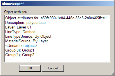
The following procedure displays some attributes of a single object in a dialog box. There is nothing exciting going on here so I’ll refrain from providing a step-by-step explanation.
Download and open 8_2_DisplayObjectAttributes.py.import rhinoscriptsyntax as rs
def displayobjectattributes(object_id):
source = "By Layer", "By Object", "By Parent"
data = []
data.append( "Object attributes for :"+str(object_id) )
data.append( "Description: " + rs.ObjectDescription(object_id))
data.append( "Layer: " + rs.ObjectLayer(object_id))
#data.append( "LineType: " + rs.ObjectLineType(object_id))
#data.append( "LineTypeSource: " + rs.ObjectLineTypeSource(object_id))
data.append( "MaterialSource: " + str(rs.ObjectMaterialSource(object_id)))
name = rs.ObjectName(object_id)
if not name: data.append("<Unnamed object>")
else: data.append("Name: " + name)
groups = rs.ObjectGroups(object_id)
if groups:
for i,group in enumerate(groups):
data.append( "Group(%d): %s" % i+1, group )
else:
data.append("<Ungrouped object>")
s = ""
for line in data: s += line + "\n"
rs.EditBox(s, "Object attributes", "RhinoPython")
if __name__=="__main__":
id = rs.GetObject()
displayobjectattributes(id)
8.3 Points and Pointclouds
Everything begins with points. A point is nothing more than a list of values called a coordinate. The number of values in the list corresponds with the number of dimensions of the space it resides in. Space is usually denoted with an R and a superscript value indicating the number of dimensions. (The ‘R’ stems from the world ‘real’ which means the space is continuous. We should keep in mind that a digital representation always has gaps, even though we are rarely confronted with them.)
Points in 3D space, or R3 thus have three coordinates, usually referred to as [x,y,z]. Points in R2 have only two coordinates which are either called [x,y] or [u,v] depending on what kind of two dimensional space we’re talking about. Points in R1 are denoted with a single value. Although we tend not to think of one-dimensional points as ‘points’, there is no mathematical difference; the same rules apply. One-dimensional points are often referred to as ‘parameters’ and we denote them with [t] or [p].

The image on the left shows the R3 world space, it is continuous and infinite. The x-coordinate of a point in this space is the projection (the red dotted line) of that point onto the x-axis (the red solid line). Points are always specified in world coordinates in Rhino.
R2 world space (not drawn) is the same as R3 world space, except that it lacks a z-component. It is still continuous and infinite. R2 parameter space however is bound to a finite surface as shown in the center image. It is still continuous, I.e. hypothetically there is an infinite amount of points on the surface, but the maximum distance between any of these points is very much limited. R2 parameter coordinates are only valid if they do not exceed a certain range. In the example drawing the range has been set between 0.0 and 1.0 for both [u] and [v]directions, but it could be any finite domain. A point with coordinates [1.5, 0.6] would be somewhere outside the surface and thus invalid.
Since the surface which defines this particular parameter space resides in regular R3 world space, we can always translate a parametric coordinate into a 3d world coordinate. The point [0.2, 0.4] on the surface for example is the same as point [1.8, 2.0, 4.1] in world coordinates. Once we transform or deform the surface, the R3 coordinates which correspond with [0.2, 0.4] will change. Note that the opposite is not true, we can translate any R2 parameter coordinate into a 3D world coordinate, but there are many 3D world coordinates that are not on the surface and which can therefore not be written as an R2 parameter coordinate. However, we can always project a 3D world coordinate onto the surface using the closest-point relationship. We’ll discuss this in more detail later on.
If the above is a hard concept to swallow, it might help you to think of yourself and your position in space. We usually tend to use local coordinate systems to describe our whereabouts; “I’m sitting in the third seat on the seventh row in the movie theatre”, “I live in apartment 24 on the fifth floor”, “I’m in the back seat”. Some of these are variations to the global coordinate system (latitude, longitude, elevation), while others use a different anchor point. If the car you’re in is on the road, your position in global coordinates is changing all the time, even though you remain in the same back seat ‘coordinate’.
Let’s start with conversion from R1 to R3 space. The following script will add 500 colored points to the document, all of which are sampled at regular intervals across the R1 parameter space of a curve object:
Download and open 8_3_R1CurveParameterSpace.py.import rhinoscriptsyntax as rs
def main():
curve_id = rs.GetObject("Select a curve to sample", 4, True, True)
if not curve_id: return
rs.EnableRedraw(False)
t = 0
while t<=1.0:
addpointat_r1_parameter(curve_id,t)
t+=0.002
rs.EnableRedraw(True)
def addpointat_r1_parameter(curve_id, parameter):
domain = rs.CurveDomain(curve_id)
r1_param = domain[0] + parameter*(domain[1]-domain[0])
r3point = rs.EvaluateCurve(curve_id, r1_param)
if r3point:
point_id = rs.AddPoint(r3point)
rs.ObjectColor(point_id, parametercolor(parameter))
def parametercolor(parameter):
red = 255 * parameter
if red<0: red=0
if red>255: red=255
return (red,0,255-red)
if __name__=="__main__":
main()

For no good reason whatsoever, we’ll start with the bottom most function:
| Line | Description |
|---|---|
| 24 | Standard out-of-the-box function declaration which takes a single double value. This function is supposed to return a colour which changes gradually from blue to red as parameter changes from zero to one. Values outside of the range {0.0~1.0} will be clipped. |
| 25 | The red component of the colour we're going to return is declared here and assigned the naive value of 255 times the parameter. Colour components must have a value between and including 0 and 255. If we attempt to construct a colour with lower or higher values a run-time error will spoil the party. |
| 26...27 | Here's where we make sure the party can continue unimpeded. |
| 28 | Compute the colour gradient value. If parameter equals zero we want blue (0,0,255) and if it equals one we want red (255,0,0). So the green component is always zero while blue and red see-saw between 0 and 255. |
Now, on to function AddPointAtR1Parameter(). As the name implies, this function will add a single point in 3D world space based on the parameter coordinate of a curve object. In order to work correctly this function must know what curve we’re talking about and what parameter we want to sample. Instead of passing the actual parameter which is bound to the curve domain (and could be anything) we’re passing a unitized one. I.e. we pretend the curve domain is between zero and one. This function will have to wrap the required math for translating unitized parameters into actual parameters.
Since we’re calling this function a lot (once for every point we want to add), it is actually a bit odd to put all the heavy-duty stuff inside it. We only really need to perform the overhead costs of ‘unitized parameter + actual parameter’ calculation once, so it makes more sense to put it in a higher level function. Still, it will be very quick so there’s no need to optimize it yet.
| Line | Description |
|---|---|
| 14 | Function declaration. |
| 15...16 | Get the curve domain and check for Null. It will be Null if the ID does not represent a proper curve object. The Rhino.CurveDomain() method will return an array of two doubles which indicate the minimum and maximum t-parameters which lie on the curve. |
| 18 | Translate the unitized R1 coordinate into actual domain coordinates. |
| 19 | Evaluate the curve at the specified parameter. Rhino.EvaluateCurve() takes an R1 coordinate and returns an R3 coordinate. |
| 21 | Add the point, it will have default attributes. |
| 22 | Set the custom colour. This will automatically change the color-source attribute to By Object. |
The distribution of R1 points on a spiral is not very enticing since it approximates a division by equal length segments in R3 space. When we run the same script on less regular curves it becomes easier to grasp what parameter space is all about:

Let’s take a look at an example which uses all parameter spaces we’ve discussed so far:
Download and open 8_3_EvaluateDeviation.py.import rhinoscriptsyntax as rs
def main():
surface_id = rs.GetObject("Select a surface to sample", 8, True)
if not surface_id: return
curve_id = rs.GetObject("Select a curve to measure", 4, True, True)
if not curve_id: return
points = rs.DivideCurve(curve_id, 500)
rs.EnableRedraw(False)
for point in points: evaluatedeviation(surface_id, 1.0, point)
rs.EnableRedraw(True)
def evaluatedeviation( surface_id, threshold, sample ):
r2point = rs.SurfaceClosestPoint(surface_id, sample)
if not r2point: return
r3point = rs.EvaluateSurface(surface_id, r2point[0], r2point[1])
if not r3point: return
deviation = rs.Distance(r3point, sample)
if deviation<=threshold: return
rs.AddPoint(sample)
rs.AddLine(sample, r3point)
if __name__=="__main__":
main()

This script will compare a bunch of points on a curve to their projection on a surface. If the distance exceeds one unit, a line and a point will be added.
First, the R1 points are translated into R3 coordinates so we can project them onto the surface, getting the R2 coordinate [u,v] in return. This R2 point has to be translated into R3 space as well, since we need to know the distance between the R1 point on the curve and the R2 point on the surface. Distances can only be measured if both points reside in the same number of dimensions, so we need to translate them into R3 as well.
Told you it was a piece of cake…
| Line | Description |
|---|---|
| 10 | We're using the Rhino.DivideCurve() method to get all the R3 coordinates on the curve in one go. This saves us a lot of looping and evaluating. |
| 24 | Rhino.SurfaceClosestPoint() returns an array of two doubles representing the R2 point on the surface (in {u,v} coordinates) which is closest to the sample point. |
| 27 | Rhino.EvaluateSurface() in turn translates the R2 parameter coordinate into R3 world coordinates |
| 30...38 | Compute the distance between the two points and add geometry if necessary. This function returns True if the deviation is less than one unit, False if it is more than one unit and Null if something went wrong. |
One more time just for kicks. We project the R1 parameter coordinate on the curve into 3D space (Step A), then we project that R3 coordinate onto the surface getting the R2 coordinate of the closest point (Step B). We evaluate the surface at R2, getting the R3 coordinate in 3D world space (Step C), and we finally measure the distance between the two R3 points to determine the deviation:

8.4 Lines and Polylines
You’ll be glad to learn that (poly)lines are essentially the same as point-lists. The only difference is that we treat the points as a series rather than an anonymous collection, which enables us to draw lines between them. There is some nasty stuff going on which might cause problems down the road so perhaps it’s best to get it over with quick.
There are several ways in which polylines can be manifested in openNURBS™ and thus in Rhino. There is a special polyline class which is simply a list of ordered points. It has no overhead data so this is the simplest case. It’s also possible for regular nurbs curves to behave as polylines when they have their degree set to 1. In addition, a polyline could also be a polycurve made up of line segments, polyline segments, degree=1 nurbs curves or a combination of the above. If you create a polyline using the _Polyline command, you will get a proper polyline object as the Object Properties Details dialog on the left shows:
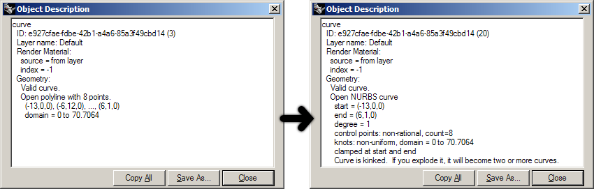
The dialog claims an “Open polyline with 8 points”. However, when we drag a control-point Rhino will automatically convert any curve to a Nurbs curve, as the image on the right shows. It is now an open nurbs curve of degree=1. From a geometric point of view, these two curves are identical. From a programmatic point of view, they are anything but. For the time being we will only deal with ‘proper’ polylines though; lists of sequential coordinates. For purposes of clarification I’ve added two example functions which perform basic operations on polyline point-lists.
Download and open 8_4_GeodesicCurve.py.Compute the length of a polyline point-array:
def PolylineLength(arrVertices):
    PolylineLength = 0.0
    for i in range(0,len(arrVertices)-1):
        PolylineLength = PolylineLength + rs.Distance(arrVertices[i], arrVertices[i+1])
Subdivide a polyline by adding extra vertices halfway between all existing vertices:
def SubDividePolyline(arrV)
    arrSubD = []

    for i in range(0, len(arrV)-1):
        'copy the original vertex location
        arrSubD.append(arrV[i])
        'compute the average of the current vertex and the next one
        arrSubD.append([arrV[i][0] + arrV[i+1][0]] / 2.0, _
                                    [arrV(i][1] + arrV[i+1][1]] / 2.0, _
                                    [arrV[i][2] + arrV[i+1][2]] / 2.0])

    'copy the last vertex (this is skipped by the loop)
    arrSubD.append(arrV[len(arrV)])
    return arrSubD
No rocket science yet, but brace yourself for the next bit…

As you know, the shortest path between two points is a straight line. This is true for all our space definitions, from R1 to RN. However, the shortest path in R2 space is not necessarily the same shortest path in R3 space. If we want to connect two points on a surface with a straight line in R2, all we need to do is plot a linear course through the surface [u,v] space. (Since we can only add curves to Rhino which use 3D world coordinates, we’ll need a fair amount of samples to give the impression of smoothness.) The thick red curve in the adjacent illustration is the shortest path in R2 parameter space connecting [A] and [B]. We can clearly see that this is definitely not the shortest path in R3 space.
We can clearly see this because we’re used to things happening in R3 space, which is why this whole R2/R3 thing is so thoroughly counter intuitive to begin with. The green, dotted curve is the actual shortest path in R3 space which still respects the limitation of the surface (I.e. it can be projected onto the surface without any loss of information). The following function was used to create the red curve; it creates a polyline which represents the shortest path from [A] to [B] in surface parameter space:
def getr2pathonsurface(surface_id, segments, prompt1, prompt2):
    start_point = rs.GetPointOnSurface(surface_id, prompt1)
    if not start_point: return

    end_point = rs.GetPointOnSurface(surface_id, prompt2)
    if not end_point: return

    if rs.Distance(start_point, end_point)==0.0: return

    uva = rs.SurfaceClosestPoint(surface_id, start_point)
    uvb = rs.SurfaceClosestPoint(surface_id, end_point)

    path = []
    for i in range(segments):
        t = i / segments
        u = uva[0] + t*(uvb[0] - uva[0])
        v = uva[1] + t*(uvb[1] - uva[1])
        pt = rs.EvaluateSurface(surface_id, u, v)
        path.append(pt)
    return path
| Line | Description |
|---|---|
| 1 | This function takes four arguments; the ID of the surface onto which to plot the shortest route, the number of segments for the path polyline and the prompts to use for picking the A and B point. |
| 1...3 | Prompt the user for the {A} point on the surface. Return if the user does not enter a point. |
| 5...6 | Prompt the user for the {B} point on the surface. Return if the user does not enter a point. |
| 10...11 | Project {A} and {B} onto the surface to get the respective R2 coordinates uva and uvb. |
| 13 | Declare the list which is going to store all the polyline vertices. |
| 14 | Since this algorithm is segment-based, we know in advance how many vertices the polyline will have and thus how often we will have to sample the surface. |
| 15 | t is a value which ranges from 0.0 to 1.0 over the course of our loop |
| 16...17 | Use the current value of t to sample the surface somewhere in between uvA and uvB. |
| 18 | rs.EvaluateSurface() takes a {u} and a {v} value and spits out a 3D-world coordinate. This is just a friendly way of saying that it converts from R2 to R3. |
We’re going to combine the previous examples in order to make a real geodesic path routine in Rhino. This is a fairly complex algorithm and I’ll do my best to explain to you how it works before we get into any actual code.
First we’ll create a polyline which describes the shortest path between [A] and [B] in R2 space. This is our base curve. It will be a very coarse approximation, only ten segments in total. We’ll create it using the function on page 54. Unfortunately that function does not take closed surfaces into account. In the paragraph on nurbs surfaces we’ll elaborate on this.
Once we’ve got our base shape we’ll enter the iterative part. The iteration consists of two nested loops, which we will put in two different functions in order to avoid too much nesting and indenting. We’re going to write four functions in addition to the ones already discussed in this paragraph:
- The main geodesic routine
- ProjectPolyline()
- SmoothPolyline()
- GeodesicFit()
The purpose of the main routine is the same as always; to collect the initial data and make sure the script completes as successfully as possible. Since we’re going to calculate the geodesic curve between two points on a surface, the initial data consists only of a surface ID and two points in surface parameter space. The algorithm for finding the geodesic curve is a relatively slow one and it is not very good at making major changes to dense polylines. That is why we will be feeding it the problem in bite-size chunks. It is because of this reason that our initial base curve (the first bite) will only have ten segments. We’ll compute the geodesic path for these ten segments, then subdivide the curve into twenty segments and recompute the geodesic, then subdivide into 40 and so on and so forth until further subdivision no longer results in a shorter overall curve.
The ProjectPolyline() function will be responsible for making sure all the vertices of a polyline point-array are in fact coincident with a certain surface. In order to do this it must project the R3 coordinates of the polyline onto the surface, and then again evaluate that projection back into R3 space. This is called ‘pulling’.
The purpose of SmoothPolyline() will be to average all polyline vertices with their neighbours. This function will be very similar to our previous example, except it will be much simpler since we know for a fact we’re not dealing with nurbs curves here. We do not need to worry about knots, weights, degrees and domains.
GeodesicFit() is the essential geodesic routine. We expect it to deform any given polyline into the best possible geodesic curve, no matter how coarse and wrong the input is. The algorithm in question is a very naive solution to the geodesic problem and it will run much slower than Rhinos native _ShortPath command. The upside is that our script, once finished, will be able to deal with self-intersecting surfaces.
The underlying theory of this algorithm is synonymous with the simulation of a contracting rubber band, with the one difference that our rubber band is not allowed to leave the surface. The process is iterative and though we expect every iteration to yield a certain improvement over the last one, the amount of improvement will diminish as we near the ideal solution. Once we feel the improvement has become negligible we’ll abort the function.
In order to simulate a rubber band we require two steps; smoothing and projecting. First we allow the rubber band to contract (it always wants to contract into a straight line between [A] and [B]). This contraction happens in R3 space which means the vertices of the polyline will probably end up away from the surface. We must then re-impose these surface constraints. These two operations have been hoisted into functions #2 and #3.

The illustration depicts the two steps which compose a single iteration of the geodesic routine. The black polyline is projected onto the surface giving the red polyline. The red curve in turn is smoothed into the green curve. Note that the actual algorithm performs these two steps in the reverse order; smoothing first, projection second.
We’ll start with the simplest function:
def projectpolyline(vertices, surface_id):
    polyline = []
    for vertex in vertices:
        pt = rs.BrepClosestPoint(surface_id, vertex)
        if pt: polyline.append(pt[0])
    return polyline
| Line | Description |
|---|---|
| 1...3 | Since this is a specialized def which we will only be using inside this script, we can skip projecting the first and last point. We can safely assume the polyline is open and that both endpoints will already be on the curve. |
| 4 | We ask Rhino for the closest point on the surface object given our polyline vertex coordinate. The reason why we do not use rs.SurfaceClosestPoint() is because BRepClosestPoint() takes trims into account. This is a nice bonus we can get for free. The native _ShortPath command does not deal with trims at all. We are of course not interested in aping something which already exists, we want to make something better. |
| 5 | If BRepClosestPoint() returned Null something went wrong after all. We cannot project the vertex in this case so we'll simply ignore it. We could of course short-circuit the whole operation after a failure like this, but I prefer to press on and see what comes out the other end. |
| 6 | The BRepClosestPoint() method returns a lot of information, not just the R2 coordinate. In fact it returns a tuple of data, the first element of which is the R3 closest point. This means we do not have to translate the uv coordinate into xyz ourselves. Huzzah! Assign it to the vertex and move on. |
def smoothpolyline(vertices):
    smooth = []
    smooth.append(vertices[0])

    for i in range(1, len(vertices)-1):
        prev = vertices[i-1]
        this = vertices[i]
        next = vertices[i+1]
        pt = (prev+this+next) / 3.0
        smooth.append(pt)
    smooth.append(vertices[len(vertices)-1])
    return smooth
| Line | Description |
|---|---|
| 1...3 6...8 | Since we need the original coordinates throughout the smoothing operation we cannot deform it directly. That is why we need to make a copy of each vertex point before we start messing about with coordinates. |
| 9 | What we do here is average the x, y and z coordinates of the current vertex ('current' as defined by i) using both itself and its neighbours.
We iterate through all the internal vertices and add the Point3d objects together, rather than explicitly adding their x, y and z components together. Writing smaller functions will not make the code go faster, but it does mean we just get to write less junk. Also, it means adjustments are easier to make afterwards since less code-rewriting is required. |
Time for the bit that sounded so difficult on the previous page, the actual geodesic curve fitter routine:
def geodesicfit(vertices, surface_id, tolerance):
    length = polylinelength(vertices)
    while True:
        vertices = smoothpolyline(vertices)
        vertices = projectpolyline(vertices, surface_id)
        newlength = polylinelength(vertices)
        if abs(newlength-length)<tolerance: return vertices
        length = newlength
| Line | Description |
|---|---|
| 1 | Hah... that doesn't look so bad after all, does it? You'll notice that it's often the stuff which is easy to explain that ends up taking a lot of lines of code. Rigid mathematical and logical structures can typically be coded very efficiently. |
| 2 | We'll be monitoring the progress of each iteration and once the curve no longer becomes noticeably shorter (where 'noticeable' is defined by the tolerance argument), we'll call the 'intermediate result' the 'final result' and return execution to the caller. In order to monitor this progress, we need to remember how long the curve was before we started; length is created for this purpose. |
| 3 | Whenever you see a while True: without any standard escape clause you should be on your toes. This is potentially an infinite loop. I have tested it rather thoroughly and have been unable to make it run more than 120 times. Experimental data is never watertight proof, the routine could theoretically fall into a stable state where it jumps between two solutions. If this happens, the loop will run forever.
You are of course welcome to add additional escape clauses if you deem that necessary. |
| 4...5 | Place the calls to the functions on page 56. These are the bones of the algorithm. |
| 6 | Compute the new length of the polyline. |
| 7 | Check to see whether or not it is worth carrying on. |
| 8 | Apparently it was, we need now to remember this new length as our frame of reference. |
The main subroutine takes some explaining. It performs a lot of different tasks which always makes a block of code harder to read. It would have been better to split it up into more discrete chunks, but we’re already using seven different functions for this script and I feel we are nearing the ceiling. Remember that splitting problems into smaller parts is a good way to organize your thoughts, but it doesn’t actually solve anything. You’ll need to find a good balance between splitting and lumping.
def geodesiccurve():
    surface_id = rs.GetObject("Select surface for geodesic curve solution", 8, True, True)
    if not surface_id: return

    vertices = getr2pathonsurface(surface_id, 10, "Start of geodesic curve", "End of geodesic curve")
    if not vertices: return

    tolerance = rs.UnitAbsoluteTolerance() / 10
    length = 1e300
    newlength = 0.0

    while True:
        print("Solving geodesic fit for %d samples" % len(vertices))
        vertices = geodesicfit(vertices, surface_id, tolerance)

        newlength = polylinelength(vertices)
        if abs(newlength-length)<tolerance: break
        if len(vertices)>1000: break
        vertices = subdividepolyline(vertices)
        length = newlength

    rs.AddPolyline(vertices)
    print("Geodesic curve added with length: ", newlength)
| Line | Description |
|---|---|
| 2...3 | Get the surface to be used in the geodesic routine. |
| 5...6 | Declare a variable which will store the polyline vertices. Since the return value of getr2pathonsurface() is already a list, we do not need to declare it with empty brackets - '[ ]' - as we have done elsewhere. |
| 8 | The tolerance used in our script will be 10% of the absolute tolerance of the document. |
| 9...12 | This loop also uses a length comparison in order to determine whether or not to continue. But instead of evaluating the length of a polyline before and after a smooth/project iteration, it measures the difference before and after a subdivide/geodesicfit iteration. The goal of this evaluation is to decide whether or not further elaboration will pay off. The variables length and newlength are used in the same context as on the previous page. |
| 13 | Display a message in the command-line informing the user about the progress we're making. This script may run for quite some time so it's important not to let the user think the damn thing has crashed. |
| 14 | Place a call to the GeodesicFit() subroutine. |
| 16...17 | Compare the improvement in length, exit the loop when there's no progress of any value. |
| 18 | A safety-switch. We don't want our curve to become too dense. |
| 19 | A call to subdividepolyline() will double the amount of vertices in the polyline. The newly added vertices will not be on the surface, so we must make sure to call geodesicfit() at least once before we add this new polyline to the document. |
| 22...23 | Add the curve and print a message about the length. |
8.5 Planes
Planes are not genuine objects in Rhino, they are used to define a coordinate system in 3D world space. In fact, it’s best to think of planes as vectors, they are merely mathematical constructs. Although planes are internally defined by a parametric equation, I find it easiest to think of them as a set of axes:

A plane definition is an array of one point and three vectors, the point marks the origin of the plane and the vectors represent the three axes. There are some rules to plane definitions, I.e. not every combination of points and vectors is a valid plane. If you create a plane using one of the RhinoScriptSyntax plane methods you don’t have to worry about this, since all the bookkeeping will be done for you. The rules are as follows:
- The axis vectors must be unitized (have a length of 1.0).
- All axis vectors must be perpendicular to each other.
- The x and y axis are ordered anti-clockwise.
The illustration shows how rules #2 and #3 work in practice.
Download and open 8_5_PlaneExample.py.ptOrigin = rs.GetPoint("Plane origin")
ptX = rs.GetPoint("Plane X-axis", ptOrigin)
ptY = rs.GetPoint("Plane Y-axis", ptOrigin)
dX = rs.Distance(ptOrigin, ptX)
dY = rs.Distance(ptOrigin, ptY)
arrPlane = rs.PlaneFromPoints(ptOrigin, ptX, ptY)
rs.AddPlaneSurface(arrPlane, 1.0, 1.0)
rs.AddPlaneSurface(arrPlane, dX, dY)

You will notice that all RhinoScriptSyntax methods that require plane definitions make sure these demands are met, no matter how poorly you defined the input.
The adjacent illustration shows how the rs.AddPlaneSurface() call on line 11 results in the red plane, while the rs.AddPlaneSurface() call on line 12 creates the yellow surface which has dimensions equal to the distance between the picked origin and axis points.
We’ll only pause briefly at plane definitions since planes, like vectors, are usually only constructive elements. In examples to come they will be used extensively so don’t worry about getting the hours in. A more interesting script which uses the rs.AddPlaneSurface() method is the one below which populates a surface with so-called surface frames:
Download and open 8_5_WhoFramedTheSurface.py. surface_id = rs.GetObject("Surface to frame", 8, True, True)
if not surface_id: return
count = rs.GetInteger("Number of iterations per direction", 20, 2)
if not count: return
udomain = rs.SurfaceDomain(surface_id, 0)
vdomain = rs.SurfaceDomain(surface_id, 1)
ustep = (udomain[1] - udomain[0]) / count
vstep = (vdomain[1] - vdomain[0]) / count
rs.EnableRedraw(False)
u = udomain[0]
while u<=udomain[1]:
v = vdomain[0]
while v<=vdomain[1]:
pt = rs.EvaluateSurface(surface_id, u, v)
if rs.Distance(pt, rs.BrepClosestPoint(surface_id, pt)[0])<0.1:
srf_frame = rs.SurfaceFrame(surface_id, [u, v])
rs.AddPlaneSurface(srf_frame, 1.0, 1.0)
v+=vstep
u+=ustep
rs.EnableRedraw(True)
Frames are planes which are used to indicate geometrical directions. Both curves, surfaces and textured meshes have frames which identify tangency and curvature in the case of curves and [u] and [v] directions in the case of surfaces and meshes. The script above simply iterates over the [u] and [v] directions of any given surface and adds surface frame objects at all uv coordinates it passes.

On lines 9 and 10 we determine the domain of the surface in u and v directions and we derive the required stepsize from those limits.
Line 14 and 16 form the main structure of the two-dimensional iteration. You can read such nested For loops as “Iterate through all columns and inside every column iterate through all rows”.
Line 18 does something interesting which is not apparent in the adjacent illustration. When we are dealing with trimmed surfaces, those two lines prevent the script from adding planes in cut-away areas. By comparing the point on the (untrimmed) surface to it’s projection onto the trimmed surface, we know whether or not the [uv] coordinate in question represents an actual point on the trimmed surface.
The rs.SurfaceFrame() method returns a unitized frame whose axes point in the [u] and [v] directions of the surface. Note that the [u] and [v] directions are not necessarily perpendicular to each other, but we only add valid planes whose x and y axis are always at 90º, thus we ignore the direction of the v-component.
8.6 Circles, Ellipses and Arcs
Although the user is never confronted with parametric objects in Rhino, the openNURBS™ kernel has a certain set of mathematical primitives which are stored parametrically. Examples of these are cylinders, spheres, circles, revolutions and sum-surfaces. To highlight the difference between explicit (parametric) and implicit circles:

When adding circles to Rhino through scripting, we can either use the Plane+Radius approach or we can use a 3-Point approach (which is internally translated into Plane+Radius). You may remember that circles are tightly linked with sines and cosines; those lovable, undulating waves. We’re going to create a script which packs circles with a predefined radius onto a sphere with another predefined radius. Now, before we start and I give away the answer, I’d like you to take a minute and think about this problem.
The most obvious solution is to start stacking circles in horizontal bands and simply to ignore any vertical nesting which might take place. If you reached a similar solution and you want to keep feeling good about yourself I recommend you skip the following two sentences. This very solution has been found over and over again but for some reason Dave Rusin is usually given as the inventor. Even though Rusin’s algorithm isn’t exactly rocket science, it is worth discussing the mathematics in advance to prevent -or at least reduce- any confusion when I finally confront you with the code.
Rusin’s algorithm works as follows:
- Solve how many circles you can evenly stack from north pole to south pole on the sphere.
- For each of those bands, solve how many circles you can stack evenly around the sphere.
- Do it.
No wait, back up. The first thing to realize is how a sphere actually works. Only once we master spheres can we start packing them with circles. In Rhino, a sphere is a surface of revolution, which has two singularities and a single seam:

The north pole (the black dot in the left most image) and the south pole (the white dot in the same image) are both on the main axis of the sphere and the seam (the thick edge) connects the two. In essence, a sphere is a rectangular plane bent in two directions, where the left and right side meet up to form the seam and the top and bottom edge are compressed into a single point each (a singularity). This coordinate system should be familiar since we use the same one for our own planet. However, our planet is divided into latitude and longitude degrees, whereas spheres are defined by latitude and longitude radians. The numeric domain of the latitude of the sphere starts in the south pole with -½π, reaches 0.0 at the equator and finally terminates with ½π at the north pole. The longitudinal domain starts and stops at the seam and travels around the sphere from 0.0 to 2π. Now you also know why it is called a ‘seam’ in the first place; it’s where the domain suddenly jumps from one value to another, distant one.

We cannot pack circles in the same way as we pack squares in the image above since that would deform them heavily near the poles, as indeed the squares are deformed. We want our circles to remain perfectly circular which means we have to fight the converging nature of the sphere
Assuming the radius of the circles we are about to stack is sufficiently smaller than the radius of the sphere, we can at least place two circles without thinking; one on the north- and one on the south pole. The additional benefit is that these two circles now handsomely cover up the singularities so we are only left with the annoying seam. The next order of business then, is to determine how many circles we need in order to cover up the seam in a straightforward fashion. The length of the seam is half of the circumference of the sphere (see yellow arrow in adjacent illustration).
Home stretch time, we’ve collected all the information we need in order to populate this sphere. The last step of the algorithm is to stack circles around the sphere, starting at every seam-circle. We need to calculate the circumference of the sphere at that particular latitude, divide that number by the diameter of the circles and once again find the largest integer value which is smaller than or equal to that result. The equivalent mathematical notation for this is:
$$N_{count} = \left[\frac{2 \cdot R_{sphere} \cdot \cos{\phi}}{2 \cdot R_{circle}} \right]$$in case you need to impress anyone…
Download and open 8_6_0_DistributeCirclesOnSphere.py.def DistributeCirclesOnSphere():
sphere_radius = rs.GetReal("Radius of sphere", 10.0, 0.01)
if not sphere_radius: return
circle_radius = rs.GetReal("Radius of circles", 0.05*sphere_radius, 0.001, 0.5*sphere_radius)
if not circle_radius: return
vertical_count = int( (math.pi*sphere_radius)/(2*circle_radius) )
rs.EnableRedraw(False)
phi = -0.5*math.pi
phi_step = math.pi/vertical_count
while phi<0.5*math.pi:
horizontal_count = int( (2*math.pi*math.cos(phi)*sphere_radius)/(2*circle_radius) )
if horizontal_count==0: horizontal_count=1
theta = 0
theta_step = 2*math.pi/horizontal_count
while theta<2*math.pi-1e-8:
circle_center = (sphere_radius*math.cos(theta)*math.cos(phi),
sphere_radius*math.sin(theta)*math.cos(phi), sphere_radius*math.sin(phi))
circle_normal = rs.PointSubtract(circle_center, (0,0,0))
circle_plane = rs.PlaneFromNormal(circle_center, circle_normal)
rs.AddCircle(circle_plane, circle_radius)
theta += theta_step
phi += phi_step
rs.EnableRedraw(True)

| Line | Description |
|---|---|
| 1...6 | Collect all custom variables and make sure they make sense. We don't want spheres smaller than 0.01 units and we don't want circle radii larger than half the sphere radius. |
| 8 | Compute the number of circles from pole to pole. The int() function in VBScript takes a double and returns only the integer part of that number. Hence it always rounds downwards. |
| 11...12 16...17 |
phi and theta (Φ and Θ) are typically used to denote angles in spherical space and it's not hard to see why. I could have called them latitude and longitude respectively as well. |
| 13 | The phi loop runs from -½π to ½π and we need to run it VerticalCount times. |
| 14 | This is where we calculate how many circles we can fit around the sphere on the current latitude. The math is the same as before, except we also need to calculate the length of the path around the sphere: 2π·R·Cos(Φ) |
| 15 | If it turns out that we can fit no circles at all at a certain latitude, we're going to get into trouble since we use the HorizontalCount variable as a denominator in the stepsize calculation on line 24. And even my mother knows you cannot divide by zero. However, we know we can always fit at least one circle. |
| 18 | This loop is essentially the same as the one on line 20, except it uses a different stepsize and a different numeric range ({0.0 <= theta < 2π} instead of {-½π <= phi <= +½π}). The more observant among you will have noticed that the domain of theta reaches from nought up to but not including two pi. If theta would go all the way up to 2π then there would be a duplicate circle on the seam. The best way of preventing a loop to reach a certain value is to subtract a fraction of the stepsize from that value, in this case I have simply subtracted a ludicrously small number (1e-8 = 0.00000001). |
| 19...21 | circle_center will be used to store the center point of the circles we're going to add. circle_normal will be used to store the normal of the plane in which these circles reside. circle_plane will be used to store the resulting plane definition. |
| 19 | This is mathematically the most demanding line, and I'm not going to provide a full proof of why and how it works. This is the standard way of translating the spherical coordinates Φ and Θ into Cartesian coordinates x, y and z.
Further information can be found on [MathWorld.com](http://mathworld.wolfram.com/) |
| 20 | Once we found the point on the sphere which corresponds to the current values of phi and theta, it's a piece of proverbial cake to find the normal of the sphere at that location. The normal of a sphere at any point on its surface is the inverted vector from that point to the center of the sphere. And that's what we do on line 29, we subtract the sphere origin (always (0,0,0) in this script) from the newly found {x,y,z} coordinate. |
| 21...22 | We can construct a plane definition from a single point on that plane and a normal vector and we can construct a circle from a plane definition and a radius value. Voila. |
8.6.1 Ellipses
Ellipses essentially work the same as circles, with the difference that you have to supply two radii instead of just one. Because ellipses only have two mirror symmetry planes and circles possess rotational symmetry (I.e. an infinite number of mirror symmetry planes), it actually does matter a great deal how the base-plane is oriented in the case of ellipses. A plane specified merely by origin and normal vector is free to rotate around that vector without breaking any of the initial constraints.
The following example script demonstrates very clearly how the orientation of the base plane and the ellipse correspond. Consider the standard curvature analysis graph as shown on the left:

It gives a clear impression of the range of different curvatures in the spline, but it doesn’t communicate the helical twisting of the curvature very well. Parts of the spline that are near-linear tend to have a garbled curvature since they are the transition from one well defined bend to another. The arrows in the left image indicate these areas of twisting but it is hard to deduce this from the curvature graph alone. The upcoming script will use the curvature information to loft a surface through a set of ellipses which have been oriented into the curvature plane of the local spline geometry. The ellipses have a small radius in the bending plane of the curve and a large one perpendicular to the bending plane. Since we will not be using the strength of the curvature but only its orientation, small details will become very apparent.
Download and open 8_6_1_FlatWorm.py.def FlatWorm():
curve_object = rs.GetObject("Pick a backbone curve", 4, True, False)
if not curve_object: return
samples = rs.GetInteger("Number of cross sections", 100, 5)
if not samples: return
bend_radius = rs.GetReal("Bend plane radius", 0.5, 0.001)
if not bend_radius: return
perp_radius = rs.GetReal("Ribbon plane radius", 2.0, 0.001)
if not perp_radius: return
crvdomain = rs.CurveDomain(curve_object)
crosssections = []
t_step = (crvdomain[1]-crvdomain[0])/samples
t = crvdomain[0]
while t<=crvdomain[1]:
crvcurvature = rs.CurveCurvature(curve_object, t)
crosssectionplane = None
if not crvcurvature:
crvPoint = rs.EvaluateCurve(curve_object, t)
crvTangent = rs.CurveTangent(curve_object, t)
crvPerp = (0,0,1)
crvNormal = rs.VectorCrossProduct(crvTangent, crvPerp)
crosssectionplane = rs.PlaneFromFrame(crvPoint, crvPerp, crvNormal)
else:
crvPoint = crvcurvature[0]
crvTangent = crvcurvature[1]
crvPerp = rs.VectorUnitize(crvcurvature[4])
crvNormal = rs.VectorCrossProduct(crvTangent, crvPerp)
crosssectionplane = rs.PlaneFromFrame(crvPoint, crvPerp, crvNormal)
if crosssectionplane:
csec = rs.AddEllipse(crosssectionplane, bend_radius, perp_radius)
crosssections.append(csec)
t += t_step
if not crosssections: return
rs.AddLoftSrf(crosssections)
rs.DeleteObjects(crosssections)
| Line | Description |
|---|---|
| 16 | crosssections is a list where we will store all our ellipse IDs. We need to remember all the ellipses we add since they have to be fed to the rs.AddLoftSrf() method. crosssectionplane will contain the base plane data for every individual ellipse, we do not need to remember these planes so we can afford to overwrite the old value with any new one. You'll notice I'm violating a lot of naming conventions from paragraph [2.3.5 Using Variables]. If you want to make something of it we can take it outside. |
| 19 | We'll be walking along the curve with equal parameter steps. This is arguably not the best way, since we might be dealing with a polycurve which has wildly different parameterizations among its subcurves. This is only an example script though so I wanted to keep the code to a minimum. We're using the same trick as before in the header of the loop to ensure that the final value in the domain is included in the calculation. By extending the range of the loop by one billionth of a parameter we circumvent the 'double noise problem' which might result from multiple additions of doubles. |
| 20 | The rs.CurveCurvature() method returns a whole set of data to do with curvature analysis. However, it will fail on any linear segment (the radius of curvature is infinite on linear segments). |
| 22...27 | Hence, if it fails we have to collect the standard information in the old fashioned way. We also have to pick a crvPerp vector since none is available. We could perhaps use the last known one, or look at the local plane of the curve beyond the current -unsolvable- segment, but I've chosen to simply use a z-axis vector by default. |
| 28...32 | If the curve does have curvature at t, then we extract the required information directly from the curvature data. |
| 33 | Construct the plane for the ellipse. |
| 35...37 | Add the ellipse to the file and append the new ellipse curve ID csec to the list crosssections. |
| 40...42 | Create a lofted surface through all ellipses and delete the curves afterwards. |
8.6.2 Arcs
Since the topic of Arcs isn’t much different from the topic of Circles, I thought it would be a nice idea to drag in something extra. This something extra is what we programmers call “recursion” and it is without doubt the most exciting thing in our lives (we don’t get out much). Recursion is the process of self-repetition. Like loops which are iterative and execute the same code over and over again, recursive functions call themselves and thus also execute the same code over and over again, but this process is hierarchical. It actually sounds harder than it is. One of the success stories of recursive functions is their implementation in binary trees which are the foundation for many search and classification algorithms in the world today. I’ll allow myself a small detour on the subject of recursion because I would very much like you to appreciate the power that flows from the simplicity of the technique. Recursion is unfortunately one of those things which only become horribly obvious once you understand how it works.
Imagine a box in 3D space which contains a number of points within its volume. This box exhibits a single behavioral pattern which is recursive. The recursive function evaluates a single conditional statement: {when the number of contained points exceeds a certain threshold value then subdivide into 8 smaller boxes, otherwise add yourself to the document}. It would be hard to come up with an easier If…Else statement. Yet, because this behavior is also exhibited by all newly created boxes, it bursts into a chain of recursion, resulting in the voxel spaces in the images below:

The input in these cases was a large pointcloud shaped like the upper half of a sphere. There was also a dense spot with a higher than average concentration of points. Because of the approximating pattern of the subdivision, the recursive cascade results in these beautiful stacks. Trying to achieve this result without the use of recursion would entail a humongous amount of bookkeeping and many, many lines of code. Before we can get to the cool bit we have to write some of the supporting functions, which -I hate to say it- once again involve goniometry (the mathematics of angles).
The problem: adding an arc using the start point, end point and start direction. As you will be aware there is a way to do this directly in Rhino using the mouse. In fact a brief inspection yields 14 different ways in which arcs can be drawn in Rhino manually and yet there are only two ways to add arcs through scripting:
- rs.AddArc(Plane, Radius, Angle)
- rs.AddArc3Pt(Point, Point, Point)
The first way is very similar to adding circles using plane and radius values, with the added argument for sweep angle. The second way is also similar to adding circles using a 3-point system, with the difference that the arc terminates at the first and second point. There is no direct way to add arcs from point A to point B while constrained to a start tangent vector. We’re going to have to write a function which translates the desired Start-End-Direction approach into a 3-Point approach. Before we tackle the math, let’s review how it works:

We start with two points {A} & {B} and a vector definition {D}. The arc we’re after is the red curve, but at this point we don’t know how to get there yet. Note that this problem might not have a solution if {D} is parallel or anti-parallel to the line from {A} to {B}. If you try to draw an arc like that in Rhino it will not work. Thus, we need to add some code to our function that aborts when we’re confronted with unsolvable input.
We’re going to find the coordinates of the point in the middle of the desired arc {M}, so we can use the 3Point approach with {A}, {B} and {M}. As the illustration on the left indicates, the point in the middle of the arc is also on the line perpendicular from the middle {C} of the baseline.
The halfway point on the arc also happens to lie on the bisector between {D} and the baseline vector. We can easily construct the bisector of two vectors in 3D space by process of unitizing and adding both vectors. In the illustration on the left the bisector is already pointing in the right direction, but it still hasn’t got the correct length.
We can compute the correct length using the standard “Sin-Cos-Tan right triangle rules”:
The triangle we have to solve has a 90º angle in the lower right corner, a is the angle between the baseline and the bisector, the length of the bottom edge of the triangle is half the distance between {A} and {B} and we need to compute the length of the slant edge (between {A} and {M}).
The relationship between a and the lengths of the sides of the triangle is:
$$\cos({\alpha})=\frac{0.5D}{?} \gg \frac{1}{\cos({\alpha})}=\frac{?}{0.5D} \gg \frac{0.5D}{\cos({\alpha})} = ?$$We now have the equation we need in order to solve the length of the slant edge. The only remaining problem is cos(a). In the paragraph on vector mathematics (6.2 Points and Vectors) the vector dotproduct is briefly introduced as a way to compute the angle between two vectors. When we use unitized vectors, the arccosine of the dotproduct gives us the angle between them. This means the dotproduct returns the cosine of the angle between these vectors. This is a very fortunate turn of events since the cosine of the angle is exactly the thing we’re looking for. In other words, the dotproduct saves us from having to use the cosine and arccosine functions altogether. Thus, the distance between {A} and {M} is the result of:
Download and open 8_6_2_AddArcDir.py.(0.5 * rs.Distance(A, B)) / rs.VectorDotProduct(D, Bisector)
def AddArcDir(ptStart, ptEnd, vecDir):
    vecBase = rs.PointSubtract(ptEnd, ptStart)
    if rs.VectorLength(vecBase)==0.0: return

    if rs.IsVectorParallelTo(vecBase, vecDir):
        return rs.AddLine(ptStart, ptEnd)

    vecBase = rs.VectorUnitize(vecBase)
    vecDir = rs.VectorUnitize(vecDir)

    vecBisector = rs.VectorAdd(vecDir, vecBase)
    vecBisector = rs.VectorUnitize(vecBisector)

    dotProd = rs.VectorDotProduct(vecBisector, vecDir)
    midLength = (0.5*rs.Distance(ptStart, ptEnd))/dotProd

    vecBisector = rs.VectorScale(vecBisector, midLength)
    return rs.AddArc3Pt(ptStart, rs.PointAdd(ptStart, vecBisector), ptEnd)
| Line | Description |
|---|---|
| 1 | The ptStart argument indicates the start of the arc, ptEnd the end and vecDir the direction at ptStart. This function will behave just like the rs.AddArc3Pt() method. It takes a set of arguments and returns the identifier of the created curve object if successful. If no curve was added the function does not return anything - that is, the resulting assignment will be None. |
| 2 | Create the baseline vector (from {A} to {B}), by subtracting {A} from {B}. |
| 3 | If {A} and {B} are coincident, then the subtraction from line 2 will result in a vector with a length of 0 and no solution is possible. Actually, there is an infinite number of solutions so we wouldn't know which one to pick. |
| 5 | If vecDir is parallel (or anti-parallel) to the baseline vector, then no solution is possible at all. |
| 8...9 | Make sure all vector definitions so far are unitized - that is, they all have a vector length value of one |
| 11...12 | Create the bisector vector and unitize it. |
| 14 | Compute the dotproduct between the bisector and the direction vector. Since the bisector is exactly halfway between the direction vector and baseline vector (indeed, that is the point to its existence), we could just as well have calculated the dotproduct between it and the baseline vector. |
| 15 | Compute the distance between ptStart and the center point of the desired arc. |
| 17 | Resize the (unitized) bisector vector to match this length. |
| 18 | Create an arc using the start, end and midpoint arguments, return the ID. |

We need this function in order to build a recursive tree-generator which outputs trees made of arcs. Our trees will be governed by a set of five variables but -due to the flexible nature of the recursive paradigm- it will be very easy to add more behavioral patterns. The growing algorithm as implemented in this example is very simple and doesn’t allow a great deal of variation.
Download and open 8_6_2_RecursivePlantGenerator.py.The five base parameters are:
- Propagation factor
- Twig length
- Twig length mutation
- Twig angle
- Twig angle mutation
The propagation-factor is a numeric range which indicates the minimum and maximum number of twigs that grow at the end of every branch. This is a totally random affair, which is why it is called a “factor” rather than a “number”. More on random numbers in a minute. The twig-length and twig-length-mutation variables control the -as you probably guessed- length of the twigs and how the length changes with every twig generation. The twig-angle and twig-angle-mutation work in a similar fashion.
The actual recursive bit of this algorithm will not concern itself with the addition and shape of the twig-arcs. This is done by a supporting function which we have to write before we can start growing trees. The problem we have when adding new twigs, is that we want them to connect smoothly to their parent branch. We’ve already got the plumbing in place to make tangency continuous arcs, but we have no mechanism yet for picking the end-point. In our current plant-scheme, twig growth is controlled by two factors; length and angle. However, since more than one twig might be growing at the end of a branch there needs to be a certain amount of random variation to keep all the twigs from looking the same.

The adjacent illustration shows the algorithm we’ll be using for twig propagation. The red curve is the branch-arc and we need to populate the end with any number of twig-arcs. Point {A} and Vector {D} are dictated by the shape of the branch but we are free to pick point {B} at random provided we remain within the limits set by the length and angle constraints. The complete set of possible end-points is drawn as the yellow cone. We’re going to use a sequence of Vector methods to get a random point {B} in this shape:
- Create a new vector {T} parallel to {D}
- Resize {T} to have a length between {Lmin} and {Lmax}
- Mutate {T} to deviate a bit from {D}
- Rotate {T} around {D} to randomize the orientation
def RandomPointInCone( origin, direction, minDistance, maxDistance, maxAngle):
    vecTwig = rs.VectorUnitize(direction)
    vecTwig = rs.VectorScale(vecTwig, minDistance + random.random()*(maxDistance-minDistance))
    MutationPlane = rs.PlaneFromNormal((0,0,0), vecTwig)
    vecTwig = rs.VectorRotate(vecTwig, random.random()*maxAngle, MutationPlane[1])
    vecTwig = rs.VectorRotate(vecTwig, random.random()*360, direction)
    return rs.PointAdd(origin, vecTwig)
| Line | Description |
|---|---|
| 1 | origin is synonymous with point {A}. direction is synonymous with vector {D}. minDistance and MaxDistance indicate the length-wise domain of the cone. maxAngle is a value which specifies the angle of the cone (in degrees, not radians). |
| 2...3 | Create a new vector parallel to Direction and resize it to be somewhere between MinDistance and MaxDistance. I'm using the random() function here which is a Python pseudo-random-number frontend. It always returns a random value between zero and one. |
| 4 | In order to mutate vecTwig, we need to find a parallel vector. since we only have one vector here we cannot directly use the Rhino.VectorCrossProduct() method, so we'll construct a plane and use its x-axis. This vector could be pointing anywhere, but always perpendicular to vecTwig. |
| 5 | Mutate vecTwig by rotating a random amount of degrees around the plane x-axis. |
| 6 | Mutate vecTwig again by rotating it around the Direction vector. This time the random angle is between 0 and 360 degrees. |
| 7 | Create the new point as inferred by Origin and vecTwig. |
One of the definitions Wikipedia has to offer on the subject of recursion is: “In order to understand recursion, one must first understand recursion.” Although this is obviously just meant to be funny, there is an unmistakable truth as well. The upcoming script is recursive in every definition of the word, it is also quite short, it produces visually interesting effects and it is quite clearly a very poor realistic plant generator. The perfect characteristics for exploration by trial-and-error. Probably more than any other example script in this primer this one is a lot of fun to play around with. Modify, alter, change, mangle and bend it as you see fit.
There is a set of rules to which any working recursive function must adhere. It must place at least one call to itself somewhere before the end and must have a way of exiting without placing any calls to itself. If the first condition is not met the function cannot be called recursive and if the second condition is not met it will call itself until time stops (or rather until the call-stack memory in your computer runs dry).
Lo and behold! A mere 21 lines of code to describe the growth of an entire tree.
def RecursiveGrowth( ptStart, vecDir, props, generation):
    minTwigCount, maxTwigCount, maxGenerations, maxTwigLength, lengthMutation, maxTwigAngle,...
        angleMutation = props
    if generation>maxGenerations: return

    #Copy and mutate the growth-properties
    newProps = props
    maxTwigLength *= lengthMutation
    maxTwigAngle *= angleMutation
    if maxTwigAngle>90: maxTwigAngle=90

    #Determine the number of twigs (could be less than zero)
    newprops = minTwigCount, maxTwigCount, maxGenerations, maxTwigLength, lengthMutation,...
        maxTwigAngle, angleMutation
    maxN = int( minTwigCount+random.random()*(maxTwigCount-minTwigCount) )
    for n in range(1,maxN):
        ptGrow = RandomPointInCone(ptStart, vecDir, 0.25*maxTwigLength, maxTwigLength,...
            maxTwigAngle)
        newTwig = AddArcDir(ptStart, ptGrow, vecDir)
        if newTwig:
            vecGrow = rs.CurveTangent(newTwig, rs.CurveDomain(newTwig)[1])
            RecursiveGrowth(ptGrow, vecGrow, newProps, generation+1)
| Line | Description |
|---|---|
| 1 | A word on the function signature. Apart from the obvious arguments ptStart and vecDir, this function takes an tuple and a generation counter. The tuple contains all our growth variables. Since there are seven of them in total I didn't want to add them all as individual arguments. Also, this way it is easier to add parameters without changing function calls. The generation argument is an integer telling the function which twig generation it is in. Normally a recursive function does not need to know its depth in the grand scheme of things, but in our case we're making an exception since the number of generations is an exit threshold. |
| 2 | For readability, we will break our tuple into individual variables. On the assignment side, the variables are listed in the order that they appear in the tuple. The properties tuple consists of the following items:

|
| 3 | If the current generation exceeds the generation limit (which is stored at the third element in the properties tuple, and broken out to the variable maxGenerations) this function will abort without calling itself. Hence, it will take a step back on the recursive hierarchy. |
| 6 | This is where we make a copy of the properties. You see, when we are going to grow new twigs, those twigs will be called with mutated properties, however we require the unmutated properties inside this function instance. |
| 7...9 | Mutate the copied properties. I.e. multiply the maximum-twig-length by the twig-length-mutation factor and do the same for the angle. We must take additional steps to ensure the angle doesn't go berserk so we're limiting the mutation to within the 90 degree realm. |
| 13 | maxN is an integer which indicated the number of twigs we are about to grow. maxN is randomly picked between the two allowed extremes (Props(0) and Props(1)). The random() function generates a number between zero and one which means that maxN can become any value between and including the limits. |
| 15 | This is where we pick a point at random using the unmutated properties. The length constraints we're using is hard coded to be between the maximum allowed length and a quarter of the maximum allowed length. There is nothing in the universe which suggests a factor of 0.25, it is purely arbitrary. It does however have a strong effect on the shape of the trees we're growing. It means it is impossible to accurately specify a twig length. There is a lot of room for experimentation and change here. |
| 16 | We create the arc that belongs to this twig. |
| 17 | If the distance between ptStart and ptGrow was 0.0 or if vecDir was parallel to ptStart » ptGrow then the arc could not be added. We need to catch this problem in time. |
| 18 | We need to know the tangent at the end of the newly created arc curve. The domain of a curve consists of two values (a lower and an upper bound). Rhino.CurveDomain(newTwig)(1) will return the upper bound of the domain. This is the same as calling:
crvDomain = rs.CurveDomain(newTwig)
vecGrow = rs.CurveTangent(newTwig, crvDomain[1])
|
| 19 | Awooga! Awooga! A function calling itself! This is it! We made it! The thing to realize is that the call is now different. We're putting in different arguments which means this new function instance behaves differently than the current function instance. |
It would have been possible to code this tree-generator in an iterative (For loops) fashion. The tree would look the same even though the code would be very different (probably a lot more lines). The order in which the branches are added would very probably also have differed. The trees below are archetypal, digital trees, the one on the left generated using iteration, the one on the right generated using recursion. Note the difference in branch order. If you look carefully at the recursive function on the previous page you’ll probably be able to work out where this difference comes from…

A small comparison table for different setting combinations. Please note that the trees have a very high random component.

8.7 Nurbs-curves
Circles and arcs are all fine and dandy, but they cannot be used to draw freeform shapes. For that you need splines. The worlds most famous spline is probably the Bézier curve, which was developed in 1962 by the French engineer Pierre Bézier while he was working for Renault. Most splines used in computer graphics these days are variations on the Bézier spline, and they are thus a surprisingly recent arrival on the mathematical scene. Other ground-breaking work on splines was done by Paul de Casteljau at Citroën and Carl de Boor at General Motors. The thing that jumps out here is the fact that all these people worked for car manufacturers. With the increase in engine power and road quality, the automobile industry started to face new problems halfway through the twentieth century, one of which was aerodynamics. New methods were needed to design mass-production cars that had smooth, fluent curves as opposed to the tangency and curvature fractured shapes of old. They needed mathematically accurate, freely adjustable geometry. Enter splines.
Before we start with NURBS curves (the mathematics of which are a bit too complex for a scripting primer) I’d like to give you a sense of how splines work in general and Béziers work in particular. I’ll explain the de Casteljau algorithm which is a very straightforward way of evaluating properties of simple splines. In practice, this algorithm will rarely be used since its performance is worse than alternate approaches, but due to its visual appeal it is easier to ‘get a feel’ for it.

Splines limited to four control points were not the end of the revolution of course. Soon, more advanced spline definitions were formulated one of which is the NURBS curve. (Just to set the record straight; NURBS stands for Non-Uniform Rational [Basic/Basis] Spline and not Bézier-Spline as some people think. In fact, the Rhino help file gets it right, but I doubt many of you have read the glossary section, I only found out just now.) Bézier splines are a subset of NURBS curves, meaning that every Bézier spline can be represented by a NURBS curve, but not the other way around. Other curve types still in use today (but not available in Rhino) are Hermite, Cardinal, Catmull-Rom, Beta and Akima splines, but this is not a complete list. Hermite curves for example are used by the Bongo animation plug-in to smoothly transform objects through a number of keyframes.
In addition to control point locations, NURBS curves have additional properties such as the degree, knot-vectors and weights. I’m going to assume that you already know how weight factors work (if you don’t, it’s in the Rhino help file under [NURBS About]) so I won’t discuss them here. Instead, we’ll continue with the correlation between degrees and knot-vectors.
Every NURBS curve has a number associated with it which represents the degree. The degree of a curve is always a positive integer between and including 1 and 11. The degree of a curve is written as DN. Thus D1 is a degree one curve and D3 is a degree three curve. The table on the next page shows a number of curves with the exact same control-polygon but with different degrees. In short, the degree of a curve determines the range of influence of control points. The higher the degree, the larger the range.
As you will recall from the beginning of this section, a quadratic Bézier curve is defined by four control points. A quadratic NURBS curve however can be defined by any number of control points (any number larger than three that is), which in turn means that the entire curve consists of a number of connected pieces. The illustration below shows a D3 curve with 10 control points. All the individual pieces have been given a different color. As you can see each piece has a rather simple shape; a shape you could approximate with a traditional, four-point Bézier curve. Now you know why NURBS curves and other splines are often described as “piece-wise curves”.

The shape of the red piece is entirely dictated by the first four control points. In fact, since this is a D3 curve, every piece is defined by four control points. So the second (orange) piece is defined by points {A; B; C; D}. The big difference between these pieces and a traditional Bézier curve is that the pieces stop short of the local control polygon. Instead of going all the way to {D}, the orange piece terminates somewhere in the vicinity of {C} and gives way to the green piece. Due to the mathematical magic of spline curves, the orange and green pieces fit perfectly, they have an identical position, tangency and curvature at point 4.
As you may or may not have guessed at this point, the little circles between pieces represent the knot-vector of this curve. This D3 curve has ten control points and twelve knots (0~11). This is not a coincidence, the number of knots follows directly from the number of points and the degree:
$$K_N = P_N + (D-1)$$Where $${K_N}$$ is the knot count, $${P_N}$$ is the point count and $${D}$$ is the degree.
In the image on the previous page, the red and purple pieces do in fact touch the control polygon at the beginning and end, but we have to make some effort to stretch them this far. This effort is called “clamping”, and it is achieved by stacking a lot of knots together. You can see that the number of knots we need to collapse in order to get the curve to touch a control-point is the same as the degree of the curve:

A clamped curve always has a bunch of knots at the beginning and end (periodic curves do not, but we’ll get to that later). If a curve has knot clusters on the interior as well, then it will touch one of the interior control points and we have a kinked curve. There is a lot more to know about knots, but I suggest we continue with some simple nurbs curves and let Rhino worry about the knot vector for the time being.
8.7.1 Control-point curves

The _FilletCorners command in Rhino puts filleting arcs across all sharp kinks in a polycurve. Since fillet curves are tangent arcs, the corners have to be planar. All flat curves though can always be filleted as the image to the right shows.
The input curve {A} has nine G0 corners (filled circles) which qualify for a filleting operation and three G1 corners (empty circles) which do not. Since each segment of the polycurve has a length larger than twice the fillet radius, none of the fillets overlap and the result is a predictable curve {B}.
Since blend curves are freeform they are allowed to twist and curl as much as they please. They have no problem with non-planar segments. Our assignment for today is to make a script which inserts blend corners into polylines. We’re not going to handle polycurves (with freeform curved segments) since that would involve quite a lot of math and logic which goes beyond this simple curve introduction. This unfortunately means we won’t actually be making non-planar blend corners.
The logic of our BlendCorners script is simple:
- Iterate though all segments of the polyline.
- From the beginning of the segment $${A}$$, place an extra control point $${W_1}$$ at distance $${R}$$.
- From the end of the segment $${B}$$, place an extra control point $${W_2}$$ at distance $${R}$$.
- Put extra control-points halfway between $${A; W_1; W_2; B}$$.
- Insert a $$D^5$$ nurbs curve using those new control points.
Or, in graphic form:

The first image shows our input curve positioned on a unit grid. The shortest segment has a length of 1.0, the longest segment a length of 6.0. If we’re going to blend all corners with a radius of 0.75 (the circles in the second image) we can see that one of the edges has a conflict of overlapping blend radii.
The third image shows the original control points (the filled circles) and all blend radius control points (the empty circles), positioned along every segment with a distance of {R} from its nearest neighbor The two red control points have been positioned 0.5 units away (half the segment length) from their respective neighbours.
Finally, the last image shows all the control points that will be added in between the existing control points. Once we have an ordered array of all control points (ordered as they appear along the original polyline) we can create a $$D^5$$ curve using rs.AddCurve().
Download and open 8_7_1_BlendCorners.py.def blendcorners():
polyline_id = rs.GetObject("Polyline to blend", 4, True, True)
if not polyline_id: return
vertices = rs.PolylineVertices(polyline_id)
if not vertices: return
radius = rs.GetReal("Blend radius", 1.0, 0.0)
if radius is None: return
between = lambda a,b: (a+b)/2.0
newverts = []
for i in range(len(vertices)-1):
a = vertices[i]
b = vertices[i+1]
segmentlength = rs.Distance(a, b)
vec_segment = rs.PointSubtract(b, a)
vec_segment = rs.VectorUnitize(vec_segment)
if radius<(0.5*segmentlength):
vec_segment = rs.VectorScale(vec_segment, radius)
else:
vec_segment = rs.VectorScale(vec_segment, 0.5*segment_length)
w1 = rs.VectorAdd(a, vec_segment)
w2 = rs.VectorSubtract(b, vec_segment)
newverts.append(a)
newverts.append(between(a,w1))
newverts.append(w1)
newverts.append(between(w1,w2))
newverts.append(w2)
newverts.append(between(w2,b))
newverts.append(vertices[len(vertices)-1])
rs.AddCurve(newverts, 5)
rs.DeleteObject(polyline_id)
| Line | Description |
|---|---|
| 2...7 | These calls prompt the user for a polyline, get the polyline's vertices, and then promps the user for the radius of blending. Since David Rutten is the only one allowed to be so careless as to not check for None values (and we are not David Rutten) each of these operations is followed by a failure check. |
| 9...10 | Sometimes, an operation that is needed within a loop results in the same values in each loop iteration. In cases like this, programs can be made much more efficient, by performing these operations before entering the loop. The variables between and newverts will not be used until line 25, but obtaining them here at lines 9 and 10 will make the script much more efficient. |
| 11 | Begin a loop for each segment in the polyline. |
| 12...13 | Store A and B coordinates for easy reference. |
| 15...21 | vec_segment is a scaled vector that points from A to B with a length of radius. Calculate the vec_segment vector. Typically this vector has length radius, but if the current polyline segment is too short to contain two complete radii, then adjust the vec_segment accordingly. |
| 23...24 | Calculate W1 and W2. |
| 25...30 | Store all points (except B) in the newverts list. |
| 31 | Append the last point of the polyline to the newverts list. We've omitted B everywhere because the A of the next segment has the same location and we do not want coincident control-points. The last segment has no next segment, so we need to make sure B is included this time. |
| 32...33 | Create a new D5 nurbs curve and delete the original. |
8.7.2 Interpolated curves
When creating control-point curves it is very difficult to make them go through specific coordinates. Even when tweaking control-points this would be an arduous task. This is why commands like _HBar are so important. However, if you need a curve to go through many points, you’re better off creating it using an interpolated method rather than a control-point method. The _InterpCrv and _InterpCrvOnSrf commands allow you to create a curve that intersects any number of 3D points and both of these methods have an equivalent in RhinoScriptSyntax.
To demonstrate, we’re going to create a script that creates iso-distance-curves on surfaces rather than the standard iso-parameter-curves, or “isocurves” as they are usually called. Isocurves, thus connect all the points in surface space that share a similar u or v value. Because the progression of the domain of a surface is not linear (it might be compressed in some places and stretched in others, especially near the edges where the surface has to be clamped), the distance between isocurves is not guaranteed to be identical either.
The description of our algorithm is very straightforward, but I promise you that the actual script itself will be the hardest thing you’ve ever done.

Our script will take any base surface (image A) and extract a number of isocurves (image B). Then, every isocurve is trimmed to a specific length (image C) and the end-points are connected to give the iso-distance-curve (the red curve in image D). Note that we are using isocurves in the v-direction to calculate the iso-distance-curve in the u-direction. This way, it doesn’t matter much that the spacing of isocurves isn’t distributed equally. Also note that this method is only useful for offsetting surface edges as opposed to _OffsetCrvOnSrf which can offset any curve.
We can use the RhinoScriptSytnax methods rs.ExtractIsoCurve() and rs.AddInterpCrvOnSrf() for steps B and D, but step C is going to take some further thought. It is possible to divide the extracted isocurve using a fixed length, which will give us a whole list of points, the second of which marks the proper solution:

In the example above, the curve has been divided into equal length segments of 5.0 units each. The red point (the second item in the collection) is the answer we’re looking for. All the other points are of no use to us, and you can imagine that the shorter the distance we’re looking for, the more redundant points we get. Under normal circumstances I would not think twice and simply use the rs.DivideCurveLength() method. However, I’ll take this opportunity to introduce you to one of the most ubiquitous, popular and prevalent algorithms in the field of programming today: binary searching.
Imagine you have a list of integers which is -say- ten thousand items long and you want to find the number closest to sixteen. If this list is unordered (as opposed to sorted) , like so:
{-2, -10, 12, -400, 80, 2048, 1, 10, 11, -369, 4, -500, 1548, 8, … , 13, -344}
you have pretty much no option but to compare every item in turn and keep a record of which one is closest so far. If the number sixteen doesn’t occur in the list at all, you’ll have to perform ten thousand comparisons before you know for sure which number was closest to sixteen. This is known as a worst-case performance, the best-case performance would be a single comparison since sixteen might just happen to be the first item in the list… if you’re lucky.
The method described above is known as a list-search and it is a pretty inefficient way of searching a large dataset and since searching large datasets is something that we tend to do a lot in computer science, plenty research has gone into speeding things up. Today there are so many different search algorithms that we’ve had to put them into categories in order to keep a clear overview. However, pretty much all efficient searching algorithms rely on the input list being sorted, like so:
{-500, -400, -369, -344, -10, -2, 1, 4, 8, 10, 11, 12, 13, 80, … , 1548, 2048}
Once we have a sorted list it is possible to improve our worst case performance by orders of magnitude. For example, consider a slightly more advanced list-search algorithm which aborts the search once results start to become worse. Like the original list-search it will start at the first item {-500}, then continue to the second item {-400}. Since {-400} is closer to sixteen than {-500}, there is every reason to believe that the next item in the list is going to be closer still. This will go on until the algorithm has hit the number thirteen. Thirteen is already pretty close to sixteen but there is still some wiggle room so we cannot be absolutely sure ({14; 15; 16; 17; 18} are all closer and {19} is equally close). However, the next number in the list is {80} which is a much, worse result than thirteen. Now, since this list is sorted we can be sure that every number after {80} is going to be worse still so we can safely abort our search knowing that thirteen is the closest number. Now, if the number we’re searching for is near the beginning of the list, we’ll have a vast performance increase, if it’s near the end, we’ll have a small performance increase. On average though, the sorted-list-search is twice as fast as the old-fashioned-list-search.
Binary-searching does far better. Let us return to our actual problem to see how binary-searching works; find the point on a curve that marks a specific length along the curve. In the image below, the point we are looking for has been indicated with a small yellow tag, but of course we don’t know where it is when we begin our search. Instead of starting at the beginning of the curve, we start halfway between {tmin} and {tmax} (halfway the domain of the curve). Since we can ask Rhino what the length is of a certain curve subdomain we can calculate the length from {tmin} to {1}. This happens to be way too much, we’re looking for something less than half this length. Thus we divide the bit between {tmin} and {1} in half yet again, giving us {2}. We again measure the distance between {tmin} and {2}, and see that again we’re too high, but this time only just. We keep on dividing the remainder of the domain in half until we find a value {6} which is close enough for our purposes:

This is an example of the simplest implementation of a binary-search algorithm and the performance of binary searching is O(log n) which is a fancy way of saying that it’s fast. Really, really fast. And what’s more, when we enlarge the size of the collection we’re searching, the time taken to find an answer doesn’t increase in a similar fashion (as it does with list-searching). Instead, it becomes relatively faster and faster as the size of the collection grows. For example, if we double the size of the array we’re searching to 20,000 items, a list-search algorithm will take twice as long to find the answer, whereas a binary-searcher only takes ~1.075 times as long.
The theory of binary searching might be easy to grasp (maybe not right away, but you’ll see the beauty eventually), any practical implementation has to deal with some annoying, code-bloating aspects. For example, before we start a binary search operation, we must make sure that the answer we’re looking for is actually contained within the set. In our case, if we’re looking for a point {P} on the curve {C} which is 100.0 units away from the start of {C}, there exists no answer if {C} is shorter than 100.0 itself. Also, since we’re dealing with a parameter domain as opposed to a list of integers, we do not have an actual list showing all the possible values. This array would be too big to fit in the memory of your computer. Instead, all we have is the knowledge that any number between and including {tmin} and {tmax} is theoretically possible. Finally, there might not exist an exact answer. All we can really hope for is that we can find an answer within tolerance of the exact length. Many operations in computational geometry are tolerance bound, sometimes because of speed issues (calculating an exact answer would take far too long), sometimes because an exact answer cannot be found (there is simply no math available, all we can do is make a set of guesses each one progressively better than the last).
At any rate, here’s the binary-search script I came up with, I’ll deal with the inner workings afterwards:
Download and open 8_7_2_EquiDistanceOffset.py.def BSearchCurve(idCrv, Length, Tolerance):
Lcrv = rs.CurveLength(idCrv)
if Lcrv<Length: return
tmin = rs.CurveDomain(idCrv)[0]
tmax = rs.CurveDomain(idCrv)[1]
t0 = tmin
t1 = tmax
while True:
t = 0.5*(t1+t0)
Ltmp = rs.CurveLength(idCrv, 0, [tmin, t])
if abs(Ltmp-Length)<Tolerance: break
if Ltmp<Length: t0=t
else: t1 = t
return t
| Line | Description |
|---|---|
| 1 | Note that this is not a complete script, it is only the search function. The complete script is supplied in the article archive. This function takes a curve ID, a desired length and a tolerance. The return value is None if no solution exists (i.e. if the curve is shorter than Length) or otherwise the parameter that marks the desired length. |
| 2 | Ask Rhino for the total curve length. |
| 3 | Make sure the curve is longer than Length. If it isn't, abort. |
| 5...6 | Store the minimum and maximum parameters of this curve domain. If you're confused about me calling the Rhino.CurveDomain() function twice instead of just once and store the resulting array, you may congratulate yourself. It would indeed be faster to not call the same method twice in a row. However, since lines 7 and 8 are not inside a loop, they will only execute once which reduces the cost of the penalty. 99% of the time spend by this function is because of lines 16~25, if we're going to be zealous about speed, we should focus on this part of the code. |
| 7...8 | t0, t1 and t will be the variables used to define our current subdomain. t0 will mark the lower bound and t1 the upper bound. t will be halfway between t0 and t1. We need to start with the whole curve in mind, so t0 and t1 will be similar to tmin and tmax. |
| 9 | Since we do not know in advance how many steps our binary searcher is going to take, we have to use an infinite loop. |
| 10 | Calculate t always exactly in the middle of {t0, t1}. |
| 11 | Calculate the length of the subcurve from the start of the curve (tmin) to our current parameter (t). |
| 12 | If this length is close enough to the desired length, then we are done and we can abort the infinite loop. abs() -in case you were wondering- is a Python function that returns the absolute (non-negative) value of a number. This means that the tolerance argument works equally strong in both directions, which is what you'd usually want. |
| 13...14 | This is the magic bit. Looks harmless enough doesn't it? What we do here is adjust the subdomain based on the result of the length comparison. If the length of the subcurve {tmin, t} is shorter than Length, then we want to restrict ourself to the lower half of the old subdomain. If, on the other hand, the subcurve length is shorter than Length, then we want the upper half of the old domain. Notice how much more compact programming code is compared to English? |
| 15 | Return the solved t-parameter. |
I have unleashed this function on a smooth curve with a fairly well distributed parameter space (i.e. no sudden jumps in parameter “density”) and the results are listed below. The length of the total curve was 200.0 mm and I wanted to find the parameter for a subcurve length of 125.0 mm. My tolerance was set to 0.0001 mm. As you can see it took 18 refinement steps in the BSearchCurve() function to find an acceptable solution. Note how fast this algorithm homes in on the correct value, after just 6 steps the remaining error is less than 1%. Ideally, with every step the accuracy of the guess is doubled, in practise however you’re unlikely to see such a neat progression. In fact, if you closely examine the table, you’ll see that sometimes the new guess overshoots the solution so much it actually becomes worse than before (like between steps #9 and #10).
I’ve greyed out the subdomain bound parameters that remained identical between two adjacent steps. You can see that sometimes multiple steps in the same direction are required.

Now for the rest of the script as outlines on page 78:
def equidistanceoffset():
    srf_id = rs.GetObject("Pick surface to offset", 8, True, True)
    if not srf_id: return

    offset = rs.GetReal("Offset distance", 1.0, 0.0)
    if not offset: return

    udomain = rs.SurfaceDomain(srf_id, 0)
    ustep = (udomain[1]-udomain[0])/200
    rs.EnableRedraw(False)

    offsetvertices = []
    u = udomain[0]
    while u<=(udomain[1]+0.5*ustep):
        isocurves = rs.ExtractIsoCurve(srf_id, (u,0), 1)
        if isocurves:
            t = BSearchCurve(isocurves[0], offset, 0.001)
            if t is not None:
                offsetvertices.append(rs.EvaluateCurve(isocurves[0], t))
            rs.DeleteObjects(isocurves)
        u+=ustep

    if offsetvertices: rs.AddInterpCrvOnSrf(srf_id, offsetvertices)
    rs.EnableRedraw(True)

If I’ve done my job so far, the above shouldn’t require any explanation. All of it is straight forward scripting code.
The image on the right shows the result of the script, where offset values are all multiples of 10. The dark green lines across the green strip (between offsets 80.0 and 90.0) are all exactly 10.0 units long.
8.7.3 Geometric curve properties
Since curves are geometric objects, they possess a number of properties or characteristics which can be used to describe or analyze them. For example, every curve has a starting coordinate and every curve has an ending coordinate. When the distance between these two coordinates is zero, the curve is closed. Also, every curve has a number of control-points, if all these points are located in the same plane, the curve as a whole is planar. Some properties apply to the curve as a whole, others only apply to specific points on the curve. For example, planarity is a global property while tangent vectors are a local property. Also, some properties only apply to some curve types. So far we’ve dealt with lines, polylines, circles, ellipses, arcs and nurbs curves:

The last available curve type in Rhino is the polycurve, which is nothing more than an amalgamation of other types. A polycurve can be a series of line curves for example, in which case it behaves similarly to a polyline. But it can also be a combination of lines, arcs and nurbs curves with different degrees. Since all the individual segments have to touch each other (G0 continuity is a requirement for polycurve segments), polycurves cannot contain closed segments. However, no matter how complex the polycurve, it can always be represented by a nurbs curve. All of the above types can be represented by a nurbs curve.
The difference between an actual circle and a nurbs-curve-that-looks-like-a-circle is the way it is stored. A nurbs curve doesn’t have a Radius property for example, nor a Plane in which it is defined. It is possible to reconstruct these properties by evaluating derivatives and tangent vector and frames and so on and so forth, but the data isn’t readily available. In short, nurbs curves lack some global properties that other curve types do have. This is not a big issue, it’s easy to remember what properties a nurbs curve does and doesn’t have. It is much harder to deal with local properties that are not continuous. For example, imagine a polycurve which has a zero-length line segment embedded somewhere inside. The t-parameter at the line beginning is a different value from the t-parameter at the end, meaning we have a curve subdomain which has zero length. It is impossible to calculate a normal vector inside this domain:

This polycurve consists of five curve segments (a nurbs-curve, a zero-length line-segment, a proper line-segment, a 90° arc and another nurbs-curve respectively) all of which touch each other at the indicated t-parameters. None of them are tangency continuous, meaning that if you ask for the tangent at parameter {t3}, you might either get the tangent at the end of the purple segment or the tangent at the beginning of the green segment. However, if you ask for the tangent vector halfway between {t1} and {t2}, you get nothing. The curvature data domain has an even bigger hole in it, since both line-segments lack any curvature:

When using curve properties such as tangents, curvature or perp-frames, we must always be careful to not blindly march on without checking for property discontinuities. An example of an algorithm that has to deal with this would be the _CurvatureGraph in Rhino. It works on all curve types, which means it must be able to detect and ignore linear and zero-length segments that lack curvature.
One thing the _CurvatureGraph command does not do is insert the curvature graph objects, it only draws them on the screen. We’re going to make a script that inserts the curvature graph as a collection of lines and interpolated curves. We’ll run into several issues already outlined in this paragraph.
In order to avoid some G continuity problems we’re going to tackle the problem span by span. In case you haven’t suffered left-hemisphere meltdown yet; the shape of every knot-span is determined by a certain mathematical function known as a polynomial and is (in most cases) completely smooth. A span-by-span approach means breaking up the curve into its elementary pieces, as shown on the left:

This is a polycurve object consisting of seven pieces; lines {A; C; E}, arcs {B; D} and nurbs curves {F; G}. When we convert the polycurve to a nurbs representation we get a degree 5 nurbs curve with 62 pieces (knot-spans). Since this curve was made by joining a bunch of other curves together, there are kinks between all individual segments. A kink is defined as a grouping of identical knots on the interior of a curve, meaning that the curve actually intersects one of its interior control-points. A kink therefore has the potential to become a sharp crease in an otherwise smooth curve, but in our case all kinks connect segments that are G1 continuous. The kinks have been marked by white circles in the image on the right. As you can see there are also kinks in the middle of the arc segments {B; D}, which were there before we joined the curves together. In total this curve has ten kinks, and every kink is a grouping of five similar knot parameters (this is a D5 curve). Thus we have a sum-total of 40 zero-length knot-spans. Never mind about the math though, the important thing is that we should prepare for a bunch of zero-length spans so we can ignore them upon confrontation.
The other problem we’ll get is the property evaluation issue I talked about on the previous page. On the transition between knots the curvature data may jump from one value to another. Whenever we’re evaluating curvature data near knot parameters, we need to know if we’re coming from the left or the right.
I’m sure all of this sounds terribly complicated. In fact, I’m sure it is terribly complicated, but these things should start to make sense. It is no longer enough to understand how scripts work under ideal circumstances, by now, you should understand why there are no ideal circumstances and how that affects programming code.
Since we know exactly what we need to do in order to mimic the _CurvatureGraph command, we might as well start at the bottom. The first thing we need is a function that creates a curvature graph on a subcurve, then we can call this function with the knot parameters as sub-domains in order to generate a graph for the whole curve:

Our function will need to know the ID of the curve in question, the subdomain {t0; t1}, the number of samples it is allowed to take in this domain and the scale of the curvature graph. The return value should be a collection of object IDs which were inserted to make the graph. This means all the perpendicular red segments and the dashed black curve connecting them.
Download and open 8_7_3_CreateCurvatureGraph.py.def addcurvaturegraphsection(idCrv, t0, t1, samples, scale):
if (t1-t0)<=0.0: return
N = -1
tstep = (t1-t0)/samples
t = t0
points = []
objects = []
while t<=(t1+(0.5*tstep)):
if t>=t1:t = t1-1e-10
N += 1
cData = rs.CurveCurvature(idCrv, t)
if not cData:
points.append( rs.EvaluateCurve(idCrv, t) )
else:
c = rs.VectorScale(cData[4], scale)
a = cData[0]
b = rs.VectorSubtract(a, c)
objects.append(rs.AddLine(a,b))
points.append(b)
t += tstep
objects.append(rs.AddInterpCurve(points))
return objects
| Line | Description |
|---|---|
| 2 | Check for a null span, this happens inside kinks. |
| 4 | Determine a step size for our loop (Subdomain length / Sample count). |
| 7 | objects() will hold the IDs of the perpendicular lines, and the connecting curve. |
| 8 | Define the loop and make sure we always process the final parameter by increasing the threshold with half the step size. |
| 9 | Make sure t does not go beyond t1, since that might give us the curvature data of the next segment. |
| 13 | In case of a curvature data discontinuity, do not add a line segment but append the point on the curve at the current curve coordinate t. |
| 15...19 | Compute the A and B coordinates, append them to the appropriate array and add the line segment. |
Now, we need to write a utility function that applies the previous function to an entire curve. There’s no rocket science here, just an iteration over the knot-vector of a curve object:
def addcurvaturegraph( idCrv, spansamples, scale):
    allGeometry = []
    knots = rs.CurveKnots(idCrv)
    p=5
    for i in range(len(knots)-1):
        tmpGeometry = addcurvaturegraphsection(idCrv, knots[i], knots[i+1], spansamples, scale)
        if tmpGeometry: allGeometry.append(tmpGeometry)
    rs.AddObjectsToGroup(allGeometry, rs.AddGroup())
    return allGeometry
| Line | Description |
|---|---|
| 2 | allGeometry will be a list of all IDs generated by repetitive calls to AddCurvatureGraphSection() |
| 3 | knots is the knot vector of the nurbs representation of idCrv. |
| 5 | We want to iterate over all knot spans, meaning we have to iterate over all (except the last) knot in the knot vector. Hence the minus one at the end. |
| 6 | Place a call to addcurvaturegraphsection() and store all resulting IDs in tmpGeometry. |
| 7 | If the result of AddCurvatureGraphSection() is not Null, then append all items in tmpGeometry to allGeometry. |
| 8 | Put all created objects into a new group. |
The last bit of code we need to write is a bit more extensive than we’ve done so far. Until now we’ve always prompted for a number of values before we performed any action. It is actually far more user-friendly to present the different values as options in the command line while drawing a preview of the result.
UI code tends to be very beefy, but it rarely is complex. It’s just irksome to write because it always looks exactly the same. In order to make a solid command-line interface for your script you have to do the following:
- Reserve a place where you store all your preview geometry
- Initialize all settings with sensible values
- Create all preview geometry using the default settings
- Display the command line options
- Parse the result (be it escape, enter or an option or value string)
- Select case through all your options
- If the selected option is a setting (as opposed to options like “Cancel” or “Accept”) then display a prompt for that setting
- Delete all preview geometry
- Generate new preview geometry using the changed settings.
def createcurvaturegraph():
    curve_ids = rs.GetObjects("Curves for curvature graph", 4, False, True, True)
    if not curve_ids: return

    samples = 10
    scale = 1.0

    preview = []
    while True:
        rs.EnableRedraw(False)
        for p in preview: rs.DeleteObjects(p)
        preview = []
        for id in curve_ids:
            cg = addcurvaturegraph(id, samples, scale)
            preview.append(cg)
        rs.EnableRedraw(True)

        result = rs.GetString("Curvature settings", "Accept", ("Samples", "Scale", "Accept"))
        if not result:
            for p in preview: rs.DeleteObjects(p)
            break
        result = result.upper()
        if result=="ACCEPT": break
        elif result=="SAMPLES":
            numsamples = rs.GetInteger("Number of samples per knot-span", samples, 3, 100)
            if numsamples: samples = numsamples
        elif result=="SCALE":
            sc = rs.GetReal("Scale of the graph", scale, 0.01, 1000.0)
            if sc: scale = sc
| Line | Description |
|---|---|
| 2 | Prompt for any number of curves, we do not want to limit our script to just one curve. |
| 5...6 | Our default values are a scale factor of 1.0 and a span sampling count of 10. |
| 8 | preview() is a list that contains arrays of IDs. One for each curve in idCurves. |
| 9 | Since users are allowed to change the settings an infinite number of times, we need an infinite loop around our UI code. |
| 10...11 | First of all, delete all the preview geometry, if present. |
| 13...15 | Then, insert all the new preview geometry. |
| 28 | Once the new geometry is in place, display the command options. The array at the end of the rs.GetString() method is a list of command options that will be visible. |
| 19...21 | If the user aborts (pressed Escape), we have to delete all preview geometry and exit the sub. |
| 23...29 | If the user clicks on an option, result will be the option name. The best method IronPython implements to treat the choice is the If...Then statement shown. |
| 23 | In the case of "Accept", all we have to do is exit the sub without deleting the preview geometry. |
| 24...26 | If the picked option was "Samples", then we have to ask the user for a new sample count. If the user pressed Escape during this nested prompt, we do not abort the whole script (typical Rhino behaviour would dictate this), but instead return to the base prompt. |
| 27...29 | If the picked option was "Scale", then we have to ask the user for a new scale factor, and . If the user pressed Escape during this nested prompt, we do not abort the whole script (typical Rhino behaviour would dictate this), but instead return to the base prompt. |
8.8 Meshes
Instead of Nurbs surfaces (which would be the next logical step after nurbs curves), this chapter is about meshes. I’m going to take this opportunity to introduce you to a completely different class of geometry -officially called “polygon meshes”- which represents a radically different approach to shape.
Instead of treating a surface as a deformation of a rectangular nurbs patch, meshes are defined locally, which means that a single mesh surface can have any topology it wants. A mesh surface can even be a disjoint (not connected) compound of floating surfaces, something which is absolutely impossible with Rhino nurbs surfaces. Because meshes are defined locally, they can also store more information directly inside the mesh format, such as colors, texture-coordinates and normals. The tantalizing image below indicates the local properties that we can access via RhinoScriptSyntax. Most of these properties are optional or have default values. The only essential ones are the vertices and the faces.

It is important to understand the pros and cons of meshes over alternative surface paradigms, so you can make an informed decision about which one to use for a certain task. Most differences between meshes and nurbs are self-evident and flow from the way in which they are defined. For example, you can delete any number of polygons from the mesh and still have a valid object, whereas you cannot delete knot spans without breaking apart the nurbs geometry. There’s a number of things to consider which are not implied directly by the theory though.
- Coordinates of mesh vertices are stored as single precision numbers in Rhino in order to save memory consumption. Meshes are therefore less accurate entities than nurbs objects. This is especially notable with objects that are very small, extremely large or very far away from the world origin. Mesh objects go hay-wire sooner than nurbs objects because single precision numbers have larger gaps between them than double precision numbers (see page 6).
- Nurbs cannot be shaded, only the isocurves and edges of nurbs geometry can be drawn directly in the viewport. If a nurbs surface has to be shaded, then it has to fall back on meshes. This means that inserting nurbs surfaces into a shaded viewport will result in a significant (sometimes very significant) time lag while a mesh representation is calculated.
- Meshes in Rhino can be non-manifold, meaning that more than two faces share a single edge. Although it is not technically impossible for nurbs to behave in this way, Rhino does not allow it. Non-manifold shapes are topologically much harder to deal with. If an edge belongs to only a single face it is an exterior edge (naked), if it belongs to two faces it is considered interior.
8.8.1 Geometry vs. Topology
As mentioned before, only the vertices and faces are essential components of the mesh definition. The vertices represent the geometric part of the mesh definition, the faces represent the topological part. Chances are you have no idea what I’m talking about… allow me to explain.
According to MathWorld.com topology is “the mathematical study of the properties that are preserved through deformations, twistings, and stretching of objects.” In other words, topology doesn’t care about size, shape or smell, it only deals with the platonic properties of objects, such as “how many holes does it have?”, “how many naked edges are there?” and “how do I get from Paris to Lyon without passing any tollbooths?”. The field of topology is partly common-sense (everybody intuitively understands the basics) and partly abstract-beyond-comprehension. Luckily we’re only confronted with the intuitive part here.

If you look at the images above, you’ll see a number of surfaces that are topologically identical (except {E}) but geometrically different. You can bend shape {A} and end up with shape {B}; all you have to do is reposition some of the vertices. Then if you bend it even further you get {C} and eventually {D} where the right edge has been bend so far it touches the edge on the opposite side of the surface. It is not until you merge the edges (shape {E}) that this shape suddenly changes its platonic essence, i.e. it goes from a shape with four edges to a shape with only two edges (and these two remaining edges are now closed loops as well). Do note that shapes {D} and {E} are geometrically identical, which is perhaps a little surprising.
The vertices of a mesh object are a list of 3D point coordinates. They can be located anywhere in space and they control the size and form of the mesh. The faces on the other hand do not contain any coordinate data, they merely indicate how the vertices are to be connected:

Here you see a very simple mesh with sixteen vertices and nine faces. Commands like _Scale, _Move and _Bend only affect the vertex-list, commands like _TriangulateMesh and _SwapMeshEdge only affect the face-list, commands like _ReduceMesh and _MeshTrim affect both lists. Note that the last face {I} has its corners defined in a clockwise fashion, whereas all the other faces are defined counter-clockwise. Although this makes no geometric difference, it does affect how the mesh normals are calculated and one should generally avoid creating meshes that are cw/ccw inconsistent.
Now that we know what meshes essentially consist of, we can start making mesh shapes from scratch. All we need to do is come up with a set of matching vertex/face arrays. We’ll start with the simplest possible shape, a mesh plane consisting of a grid of vertices connected with quads. Just to keep matters marginally interesting, we’ll mutate the z-coordinates of the grid points using a user-specified mathematical function in the form of:
$$f(x, y, \Theta, \Delta) = …$$
Where the user is allowed to specify any valid mathematical function using the variables x, y, Θ and Δ. Every vertex in the mesh plane has a unique combination of x and y values which can be used to determine the z value of that vertex by evaluating the custom function (Θ and Δ are the polar coordinates of x and y). This means every vertex {A} in the plane has a coordinate {B} associated with it which shares the x and y components, but not the z component.
We’ll run into four problems while writing this script which we have not encountered before, but only two of these have to do with mesh geometry/topology:
It’s easy enough to generate a grid of points, we’ve done similar looping before where a nested loop was used to generate a grid wrapped around a cylinder. The problem this time is that it’s not enough to generate the points. We also have to generate the face-list, which is highly dependent on the row and column dimensions of the vertex list. It’s going to take a lot of logic insight to get this right (probably easiest to make a schematic first). Let us turn to the problem of generating the vertex coordinates, which is a straightforward one:
Download and open 8_8_1_MeshFunction.py.def createmeshvertices(function, fdomain, resolution):
xstep = (fdomain[1]-fdomain[0])/resolution
ystep = (fdomain[3]-fdomain[2])/resolution
v = []
x = fdomain[0]
while x <= fdomain[1]+(0.5*xstep):
y = fdomain[2]
while y<=fdomain[3]+(0.5*ystep):
z = solveequation(function, x, y)
v.append( (x,y,z) )
y += ystep
x += xstep
return v
| Line | Description |
|---|---|
| 1 | This function is to be part of the finished script. It is a very specific function which merely combines the logic of nested loops with other functions inside the same script (functions which we haven't written yet, but since we know how they are supposed to work we can pretend as though they are available already). This function takes three arguments:
|
| 2...3 | The fDomain() argument has four doubles, arranged like this: (0) Minimum x-value (1) Maximum x-value (2) Minimum y-value (3) Maximum y-value We can access those easily enough, but since the step size in x and y direction involves so much math, it's better to cache those values, so we don't repeat the same calculation over and over again. |
| 6 | Begin at the lower end of the x-domain and step through the entire domain until the maximum value has been reached. We can refer to this loop as the row-loop. |
| 8 | Begin at the lower end of the y-domain and step through the entire domain until the maximum value has been reached. We can refer to this loop as the column-loop. |
| 9 | This is where we're calling an -as of yet- non-existent function. However, I think the signature is straightforward enough to not require further explanation now. |
| 9...11 | Append the new vertex to the V list. Note that vertices are stored as a one-dimensional list, which makes accessing items at a specific (row, column) coordinate slightly cumbersome. |

Once we have our vertices, we can create the face list that connects them. Since the face-list is topology, it doesn’t matter where our vertices are in space, all that matters is how they are organized. The image on the right is the mesh schematic that I always draw whenever confronted with mesh face logic. The image shows a mesh with twelve vertices and six quad faces, which has the same vertex sequence logic as the vertex list created by the function on the previous page. The vertex counts in x and y direction are four and three respectively (Nx=4, Ny=3).
Now, every quad face has to link the four vertices in a counter-clockwise fashion. You may have noticed already that the absolute differences between the vertex indices on the corners of every quad are identical. In the case of the lower left quad {A=0; B=3; C=4; D=1}. In the case of the upper right quad {A=7; B=10; C=11; D=8}. We can define these numbers in a simpler way, which reduces the number of variables to just one instead of four: {A=?; B=(A+Ny); C=(B+1); D=(A+1)}, where Ny is the number of vertices in the y-direction. Now that we know the logic of the face corner numbers, all that is left is to iterate through all the faces we need to define and calculate proper values for the A corner:
def createmeshfaces(resolution):
    nX = resolution
    nY = resolution
    f = []
    for i in range(nX-1):
        for j in range(nY-1):
            baseindex = i*(nY+1)+j
            f.append( (baseindex, baseindex+1, baseindex+nY+2, baseindex+nY+1) )
    return f
| Line | Description |
|---|---|
| 2...3 | Cache the {Nx} and {Ny} values, they are the same in our case because we do not allow different resolutions in {x} and {y} direction. |
| 4 | Declare a list to store the faces we will create. |
| 5...6 | These two nested loops are used to iterate over the grid and define a face for each row/column combo. I.e. the two values i and j are used to define the value of the A corner for each face. |
| 7 | Instead of the nondescript "A", we're using the variable name baseIndex. This value depends on the values of both i and j. The i value determines the index of the current column and the j value indicates the current offset (the row index). |
| 8 | Define the new quad face corners using the logic stated above. |
Writing a tool which works usually isn’t enough when you write it for other people. Apart from just working, a script should also be straightforward to use. It shouldn’t allow you to enter values that will cause it to crash (come to think of it, it shouldn’t crash at all), it should not take an eternity to complete and it should provide sensible defaults. In the case of this script, the user will have to enter a function which is potentially very complex, and also four values to define the numeric domain in {x} and {y} directions. This is quite a lot of input and chances are that only minor adjustments will be made during successive runs of the script. It therefore makes a lot of sense to remember the last used settings, so they become the defaults the next time around. There’s a number of ways of storing persistent data when using scripts, each with its own advantages:

We’ll be using a *.txt file to store our data since it involves very little code and it survives a Rhino restart. An *.txt file is a textfile which stores a number of Strings in a one-level hierarchical format.
def SaveFunctionData(strFunction, fDomain, Resolution):
    file = open("MeshSettings_XY.txt", "w")
    file.write(strFunction)
    file.write("\n")
    for d in fDomain:
        file.write(str(d))
        file.write("\n")
    file.write(str(Resolution))
    file.close()
| Line | Description |
|---|---|
| 2 | This is a specialized function written specifically for this script. The signature consists only of the data it has to store. The open keyword creates a stream to the file we will be modifying. Specifying a file name without a path saves the file to the directory where the script resides. The second parameter indicates what the stream will be doing - writing in this instance. |
| 3...8 | Write all settings successively to the file. We will be writing them in a specific order - strFunction, fDomain values 0 through 3, and the Resolution. The same order will be used to recover them later. |
| 9 | This call finalizes modifications to the file, and closes it for other operations. |
The contents of the *.txt file should look something like this:

Reading data from an *.txt file is slightly more involved, because there is no guarantee the file exists yet. Indeed, the first time you run this script there won’t be a settings file yet and we need to make sure we supply sensible defaults:
def loadfunctiondata():
    try:
        file = open("MeshSettings_XY.txt", "r")
        items = file.readlines()
        file.close()
        function = str(items[0])
        domain = (float(items[1]), float(items[2]),
            float(items[3]), float(items[4]))
        resolution = int(items[5])
    except:
        function = "math.cos(math.sqrt(x**2+y**2))"
        domain = (-10.0, 10.0, -10.0, 10.0)
        resolution = 50
    return function, domain, resolution
| Line | Description |
|---|---|
| 2 10 | This function needs to handle two possible conditions, the first being the first time it is called, and the second being all successive calls. The first time, there will be no "MeshSettings_XY.txt" file, so we will need to return default values, and create one later. This statement attempts to access the "MeshSettings_XY.txt" file in lines 3 to 5, and upon failure, moves to lines 11 to 13, in order to |
| 3 | Obviously we need the exact same file name. If the file does not exist, the script will throw an exception. Not to worry, though. The try...except statement we implemented earlier will handle it, and return our default values. |
| 4 | This is where we read the data strings from the \*.txt file. |
| 6...9 | The items recovered from the \*.txt file are distributed to their respective variables in the order that they were written to the file. |
| 11...13 | If an exception was thrown, we will need to return a set of default values. These are defined here. |

We’ve now dealt with two out of four problems (mesh topology, saving and loading persistent settings) and it’s time for the big ones. In our CreateMeshVertices() procedure we’ve placed a call to a function called SolveEquation() eventhough it didn’t exist yet. SolveEquation() has to evaluate a user-defined function for a specific {x,y} coordinate which is something we haven’t done before yet. It is very easy to find the answer to the question:
“What is the value of {Sin(x) + Sin(y)} for {x=0.5} and {y=2.7} ?”
However, this involves manually writing the equation inside the script and then running it. Our script has to evaluate custom equations which are not known until after the script starts. This means in turn that the equation is stored as a String variable.
The eval statement runs a script inside a script. The eval statement takes a single String and attempts to run it as a bit of code, but nested inside the current scope. That means that you can refer to local variables inside an eval. This bit of magic is exactly what we need in order to evaluate expressions stored in Strings. We only need to make sure we set up our x, y, Θ and Δ variables prior to using eval.
The fourth big problem we need to solve has to do with nonsensical users (a certain school of thought popular among programmers claims that all users should be assumed to be nonsensical). It is possible that the custom function is not valid Python syntax, in which case the eval statement will not be able to parse it. This could be because of incomplete brackets, or because of typos in functions or a million other problems. But even if the function is syntactically correct it might still crash because of incorrect mathematics.
For example, if you try to calculate the value of Sqr(-4.0), the script crashes with the “Invalid procedure call or argument” error message. The same applies to Log(-4.0). These functions crash because there exists no answer for the requested value. Other types of mathematical problems arise with large numbers. Exp(1000) for example results in an “Overflow” error because the result falls outside the double range. Another favorite is the “Division by zero” error. The following table lists the most common errors that occur in the Python engine:

See Python’s list of Built-In Exceptions for the complete list and descriptions of each.
As you can see there’s quite a lot that can go wrong. We should be able to prevent this script from crashing, even though we do not control the entire process. We could of course try to make sure that the user input is valid and will not cause any computational problems, but it is much easier to just let the script fail and recover from a crash after it happened. We’ve used the error catching mechanism previously, but back then we were just lazy, now there is no other solution.
The try/except statement can be used in Python as a great technique for error handling. First, the user implements a statement to “Try,” if this works then the statement is executed and we are finished. Otherwise, if an exception occurs we go straight to the “except” portion. If the error matches the exception named, the portion of code within the “except” segment is executed and we continue on. If an error happens that does not match the named “exception” then an “unhandled exception” message is thrown. Note - a try statement may have many except clauses and any given except clause may have multiple exceptions it is testing for!
def solveequation( function, x, y ):
    d = 10
    angledata = rs.Angle( (0,0,0), (x,y,0))
    a = 0.0
    if angledata: a = angledata[0] * math.pi/180
    try:
        z = eval(function)
    except:
        z = 0
    return z
The amount of stuff the above bit of magic does is really quite impressive. It converts the {x; y} coordinates into polar coordinates {A; D} (for Angle and Distance), makes sure the angle is an actual value, in case both {x} and {y} turn out to be zero. It solves the equation to find the z-coordinate, and sets {z} to zero in case a the equation was unsolvable. Now that all the hard work is done, all that is left is to write the over arching function that provides the interface for this script, which I don’t think needs further explanation:
def meshfunction_xy():
    zfunc, domain, resolution = loadfunctiondata()
    zfunc = rs.StringBox( zfunc, "Specify a function f(x,y[,D,A])", "Mesh function")
    if not zfunc: return

    while True:
        prompt = "Function domain x{%f,%f} y{%f,%f} @%d" % (domain[0], domain[1], domain[2], domain[3], resolution)
        result = rs.GetString(prompt, "Insert", ("xMin","xMax","yMin","yMax","Resolution","Insert"))
        if not result: return
        result = result.upper()
        if result=="XMIN":
            f = rs.GetReal("X-Domain start", domain[0])
            if f is not None: domain[0]=f
        elif result=="XMAX":
            f = rs.GetReal("X-Domain end", domain[1])
            if f is not None: domain[1]=f
        elif result=="YMIN":
            f = rs.GetReal("Y-Domain start", domain[2])
            if f is not None: domain[2]=f
        elif result=="YMAX":
            f = rs.GetReal("Y-Domain end", domain[3])
            if f is not None: domain[3]=f
        elif result=="RESOLUTION":
            f = rs.GetInteger("Resolution of the graph", resolution)
            if f is not None: resolution=f
        elif result=="INSERT": break

    verts = createmeshvertices(zfunc, domain, resolution)
    faces = createmeshfaces(resolution)
    rs.AddMesh(verts, faces)
The default function Cos(Sqr(x^2 + y^2)) is already quite pretty, but here are some other functions to play with as well:
| Notation | Syntax | result |
|---|---|---|
| $$\cos\left(\sqrt{x^2 + y^2}\right)$$ | math.cos(math.sqrt(x*x + y*y)) |  |
| $$\sin(x) + \sin(y)$$ | math.sin(x) + math.sin(y) |  |
| $$\sin(D + A)$$ | math.sin(D+A) |  |
| $$Atn\left(\sqrt{x^2 + y^2}\right)$$ | math.atan(x*x + y*y) -or- math.atan(D) |
 |
| $$\sqrt{|x|} + \sin(y)^{16}$$ | math.sqrt(math.fabs(x))+math.pow(math.sin(y),16) |  |
| $$\sin\left(\sqrt{\min(x^2, y^2)}\right)$$ | math.sin(min(math.pow([x*x, y*y]),0.5)) |  |
| $$\left[\sin(x) + \sin(y) + x + y\right]$$ | int(math.sin(x) + math.sin(y) + x + y) |  |
| $$\log\left(\sin(x) + \sin(y) + 2.01\right)$$ | math.log(math.sin(x)+math.sin(y)+2.01) |  |
8.8.2 Shape vs. Image
The vertex and face lists of a mesh object define its form (geometry and topology) but meshes can also have local display attributes. Colors and Texture-coordinates are two of these that we can control via RhinoScriptSyntax. The color list (usually referred to as ‘False-Colors’) is an optional mesh property which defines individual colors for every vertex in the mesh. The only Rhino commands that I know of that generate meshes with false-color data are the analysis commands (_DraftAngleAnalysis, _ThicknessAnalysis, _CurvatureAnalysis and so on and so forth) but unfortunately they do not allow you to export the analysis meshes. Before we do something useful with False-Color meshes, let’s do something simple, like assigning random colours to a mesh object:
 Download and open 8_8_2_RandomMeshColours.py.
def randommeshcolors():
    mesh_id = rs.GetObject("Mesh to randomize", 32, True, True)
    if not mesh_id: return

    verts = rs.MeshVertices(mesh_id)
    faces = rs.MeshFaceVertices(mesh_id)
    colors = []
    for vert in verts:
        rgb = random()*255, random()*255, random()*255
        colors.append(rgb)
    rs.AddMesh(verts, faces, vertex_colors=colors)
    rs.DeleteObject(mesh_id)
| Line | Description |
|---|---|
| 7...11 | The False-Color array is optional, but there are rules to using it. If we decide to specify a False-Color array, we have to make sure that it has the exact same number of elements as the vertex array. After all, every vertex needs its own colour. We must also make sure that every element in the False-Color array represents a valid colour. Colours in Rhino are defined as integers which store the red, green and blue channels. The channels are defined as numbers in the range {0; 255}, and they are mashed together into a bigger number where each channel is assigned its own niche. The advantage of this is that all colours are just numbers instead of more complex data-types, but the downside is that these numbers are usually meaningless for mere mortals:
1 Lowest possible value |

Random colors may be pretty, but they are not useful. All the Rhino analysis commands evaluate a certain geometrical local property (curvature, verticality, intersection distance, etc), but none of them take surroundings into account. Let’s assume we need a tool that checks a mesh and a (poly)surface for proximity. There is nothing in Rhino that can do that out of the box. So this is actually going to be a useful script, plus we’ll make sure that the script is completely modular so we can easily adjust it to analyze other properties.
We’ll need a function who’s purpose it is to generate an array of numbers (one for each vertex in a mesh) that define some kind of property. These numbers are then in turn translated into a gradient (red for the lowest number, white for the highest number in the set) and applied as the False-Color data to a new mesh object. In our case the property is the distance from a certain vertex to the point on a (poly)surface which is closest to that vertex:


Vertex {A} on the mesh has a point associated with it {Acp} on the box and the distance between these two {DA} is a measure for proximity. This measure is linear, which means that a vertex which is twice as far away gets a proximity value which is twice as high. A linear distribution is indicated by the red line in the adjacent graph. It actually makes more intuitive sense to use a logarithmic scale (the green line), since it is far better at dealing with huge value ranges. Imagine we have a mesh whose sorted proximity value set is something like:
{0.0; 0.0; 0.0; 0.1; 0.2; 0.5; 1.1; 1.8; 2.6; … ; 9.4; 1000.0}
As you can see pretty much all the variation is within the {0.0; 10.0} range, with just a single value radically larger. Now, if we used a linear approach, all the proximity values would resolve to completely red, except for the last one which would resolve to completely white. This is not a useful gradient. When you run all the proximity values through a logarithm you end up with a much more natural distribution:

There is just one snag, the logarithm function returns negative numbers for input between zero and one. In fact, the logarithm of zero is minus-infinity, which plays havoc with all mathematics down the road since infinity is way beyond the range of numbers we can represent using doubles. And since the smallest possible distance between two points in space is zero, we cannot just apply a logarithm and expect our script to work. The solution is a simple one, add 1.0 to all distance values prior to calculating the logarithm, and all our results are nice, positive numbers.
Download and open 8_8_2_RandomMeshColours.py.def VertexValueArray(points, id):
return [DistanceTo(point, id) for point in points]
def DistanceTo(pt, id):
ptCP = rs.BrepClosestPoint(id,pt)
if ptCP:
d = rs.Distance(pt, ptCP[0])
return math.log10(d+1)
| Line | Description |
|---|---|
| 1...2 | The VertexValueArray() function is the one that creates a list of numbers for each vertex. We're giving it the mesh vertices (an array of 3D points) and the object ID of the (poly)surface for the proximity analysis. This function doesn't do much, it simply iterates through the list of points using the DistanceTo() function, and returns a list of the results. |
| 4...8 | DistanceTo() calculates the distance from pt to the projection of pt onto id. Where pt is a single 3D coordinate and id if the identifier of a (poly)surface object. It also performs the logarithmic conversion, so the return value is not the actual distance. |
And the master Sub containing all the front end and color magic:
import rhinoscriptsyntax as rs
import sys
import math

def ProximityAnalysis():
    mesh_id = rs.GetObject("Mesh for proximity analysis", 32, True, True)
    if not mesh_id: return

    brep_id = rs.GetObject("Surface for proximity test", 8+16, False, True)
    if not brep_id: return

    vertices = rs.MeshVertices(mesh_id)
    faces = rs.MeshFaceVertices(mesh_id)
    listD = VertexValueArray(vertices, brep_id)

    minD = sys.float_info.min
    maxD = sys.float_info.max
    for ct in range(len(listD)):
        if minD>listD[ct]: minD = listD[ct]
        if maxD<listD[ct]: maxD = listD[ct]

    colors = []
    for i in range(len(vertices)):
        proxFactor = (listD[i]-minD)/(maxD-minD)
        colors.append((255, 255*proxFactor, 255*proxFactor))
    rs.AddMesh(vertices, faces, vertex_colors=colors)
    rs.DeleteObject(mesh_id)
| Line | Description |
|---|---|
| 1...3 | There are a couple of import statements that may look unfamiliar here. In some scripts, the use of outside resources can come in handy. Importing the System namespace allows us to use objects from the .Net framework, such as the maximum and minimum values of all floating point variables. |
| 16...20 | Since there is not a function in the math namespace, .net, or the rhinoscriptsyntax methods to get the max and min values of an array of numbers, we will have to write some code to get the maximum and minimum values of listD. The .Net framework is a wonderful place, and for the first time, IronPython allows its use in scripts within Rhinoceros. We call the System namespace, and get the max and min values of all double-precision numbers, as a starting point. We then iterate through the items in listD, comparing each value to the current value of maxD and minD, replacing them if we happen to find a more suitable member of the list for either. Once we have iterated through the entire list, we are certain we have the max and min values. |
| 22 | Create the False-Color array.. |
| 24 | Calculate the position on the {Red~White} gradient for the current value. |
| 25 | Cook up a colour based on the proxFactor. |
8.9 Surfaces
At this point you should have a fair idea about the strengths and flexibility of mesh based surfaces. It is no surprise that many industries have made meshes their primary means of surfacing. However, meshes also have their disadvantages and this is where other surfacing paradigms come into play.
In fact, meshes (like nurbs) are a fairly recent discovery whose rise to power depended heavily on demand from the computer industry. Mathematicians have been dealing with different kinds of surface definitions for centuries and they have come up with a lot of them; surfaces defined by explicit functions, surfaces defined by implicit equations, minimal area surfaces, surfaces of revolutions, fractal surfaces and many more. Most of these types are far too abstract for your every-day modeling job, which is why most CAD packages do not implement them.
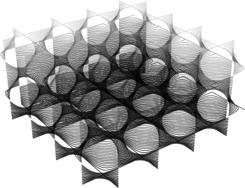
Apart from a few primitive surface types such as spheres, cones, planes and cylinders, Rhino supports three kinds of freeform surface types, the most useful of which is the Nurbs surface. Similar to curves, all possible surface shapes can be represented by a Nurbs surface, and this is the default fall-back in Rhino. It is also by far the most useful surface definition and the one we will be focusing on.

8.9.1 NURBS Surfaces

Nurbs surfaces are very similar to Nurbs curves. The same algorithms are used to calculate shape, normals, tangents, curvatures and other properties, but there are some distinct differences. For example, curves have tangent vectors and normal planes, whereas surfaces have normal vectors and tangent planes. This means that curves lack orientation while surfaces lack direction. This is of course true for all curve and surface types and it is something you’ll have to learn to live with. Often when writing code that involves curves or surfaces you’ll have to make assumptions about direction and orientation and these assumptions will sometimes be wrong.
In the case of NURBS surfaces there are in fact two directions implied by the geometry, because NURBS surfaces are rectangular grids of {u} and {v} curves. And even though these directions are often arbitrary, we end up using them anyway because they make life so much easier for us.
But lets start with something simple which doesn’t actually involve NURBS surface mathematics on our end. The problem we’re about to be confronted with is called Surface Fitting and the solution is called Error Diffusion. You have almost certainly come across this term in the past, but probably not in the context of surface geometry. Typically the words “error diffusion” are only used in close proximity to the words “color”, “pixel” and “dither”, but the wide application in image processing doesn’t limit error diffusion algorithms to the 2D realm.
The problem we’re facing is a mismatch between a given surface and a number of points that are supposed to be on it. We’re going to have to change the surface so that the distance between it and the points is minimized. Since we should be able to supply a large amount of points (and since the number of surface control-points is limited and fixed) we’ll have to figure out a way of deforming the surface in a non-linear fashion (i.e. translations and rotations alone will not get us there). Take a look at the images below which are a schematic representation of the problem:

For purposes of clarity I have unfolded a very twisted nurbs patch so that it is reduced to a rectangular grid of control-points. The diagram you’re looking at is drawn in {uvw} space rather than world {xyz} space. The actual surface might be contorted in any number of ways, but we’re only interested in the simplified {uvw} space.
The surface has to pass through point {S}, but currently the two entities are not intersecting. The projection of {S} onto the surface {S'} is a certain distance away from {S} and this distance is the error we’re going to diffuse. As you can see, {S'} is closer to some control points than others. Especially {F} and {G} are close, but {B; C; J; K} can also be considered adjacent control points. Rather than picking a fixed number of nearby control points and moving those in order to reduce the distance between {S} and {S'}, we’re going to move all the points, but not in equal amounts. The images on the right show the amount of motion we assign to each control point based on its distance to {S'}. You may have noticed a problem with the algorithm description so far. If a nurbs surface is flat, the control-points lie on the surface itself, but when the surface starts to buckle and bend, the control points have a tendency to move away from the surface. This means that the distance between the control points {uvw} coordinate and {S'} is less meaningful. So instead of control points, we’ll be using Greville points. Both nurbs curves and nurbs surfaces have a set of Greville points (or “edit points” as they are known in Rhino), but only curves expose this in the Rhino interface. As scripters we also get access to surface Greville points, which is useful because there is a 1:1 mapping between control and Greville points and the latter are guaranteed to lie on the surface. Greville points can therefore be expressed in {uv} coordinates only, which means we can also evaluate surface properties (such as tangency, normals and curvature) at these exact locations.
The only thing left undecided at this point is the equation we’re going to use to determine the amount of motion we’re going to assign to a certain control point based on its distance from {S'}. It seems obvious that all the control points that are “close” should be affected much more than those which are farther away. The minimum distance between two points in space is zero (negative distance only makes sense in certain contexts, which we’ll get to shortly) and the maximum distance is infinity. This means we need a graph that goes from zero to infinity on the x-axis and which yields a lower value for {y} for every higher value of {x}. If the graph ever goes below zero it means we’re deforming the surface with a negative error. This is not a bad thing per se, but let’s keep it simple for the time being.
Our choices are already pretty limited by these constraints, but there are still some worthy contestants. If this were a primer about mathematics I’d probably have gone for a Gaussian distribution, but instead we’ll use an extremely simple equation known as a hyperbola. If we define the diffusion factor of a Greville point as the inverse of its distance to {S'}, we get this hyperbolic function:
$$f(y)=\frac{1}{x}$$
As you can see, the domain of the graph goes from zero to infinity, and for every higher value of {x} we get a lower value of {y}, without {y} ever becoming zero. There’s just one problem, a problem which only manifests itself in programming. For very small values of {x}, when the Greville point is very close to {S'}, the resulting {y} is very big indeed. When this distance becomes zero the weight factor becomes infinite, but we’ll never get even this far. Even though the processor in your computer is in theory capable of representing numbers as large as 1.8 × 10308 (which isn’t anywhere near infinity by any stretch of the imagination), when you start doing calculations with numbers approaching the extremes chances are you are going to cross over into binary no man’s land and crash your pc. And that’s not even to mention the deplorable mathematical accuracy at these levels of scale. Clearly, you might want to steer clear of very big and very small numbers altogether.
It’s an easy fix in our case, we can simply limit the {x} value to the domain {+0.01; +∞}, meaning that {y} can never get bigger than 100. We could make this threshold much, much smaller without running into problems. Even if we limit {x} to a billionth of a unit (0.00000001) we’re still comfortably in the clear.

The first thing we need to do is write a function that takes a surface and a point in {xyz} coordinates and translates it into {uvw} coordinates. We can use the rs.SurfaceClosestPoint() method to get the {u} and {v} components, but the {w} is going to take some thinking.
First of all, a surface is a 2D entity meaning it has no thickness and thus no “real” {z} or {w} component. But a surface does have normal vectors that point away from it and which can be used to emulate a “depth” dimension. In the adjacent illustration you can see a point in {uvw} coordinates, where the value of {w} is simply the distance between the point and the start of the line. It is in this respect that negative distance has meaning, because negative distance denotes a {w} coordinate on the other side of the surface.
Although this is a useful way of describing coordinates in surface space, you should at all times remember that the {u} and {v} components are expressed in surface parameter space while the {w} component is expressed in world units. We are using mixed coordinate systems which means that we cannot blindly use distances or angles between these points because those properties are meaningless now.
In order to find the coordinates in surface {S} space of a point {P}, we need to find the projection {P'} of {P} onto {S}. Then we need to find the distance between {P} and {P'} so we know the magnitude of the {w} component and then we need to figure out on which side of the surface {P} is in order to figure out the sign of {w} (positive or negative). Since our script will be capable of fitting a surface to multiple points, we might as well make our function list-capable:
Download and open 8_9_1_fitsurface_.py. Download and open 8_9_1_surface fitter.3dm.def ConvertToUVW(idSrf, pXYZ):
pUVW = []
for point in pXYZ:
u, v = rs.SurfaceClosestPoint(idSrf, point)
surface_xyz = rs.EvaluateSurface(idSrf, u, v)
surface_normal = rs.SurfaceNormal(idSrf, (u,v))
dirPos = rs.PointAdd(surface_xyz, surface_normal)
dirNeg = rs.PointSubtract(surface_xyz, surface_normal)
dist = rs.Distance(surface_xyz, point)
if (rs.Distance(point, dirPos) > rs.Distance(point, dirNeg)): dist *= -1
pUVW.append((u, v, dist))
return pUVW
| Line | Description |
|---|---|
| 1 | pXYZ() is an array of points expressed in world coordinates. |
| 4...6 | Find the {uv} coordinate of {P'}, the {xyz} coordinates of {P'} and the surface normal vector at {P'}. |
| 8...10 | Add and subtract the normal to the {xyz} coordinates of {P'} to get two points on either side of {P'}. |
| 12...13 | If {P} is closer to the dirNeg point, we know that {P} is on the "downside" of the surface and we need to make {w} negative. |
We need some other utility functions as well (it will become clear how they fit into the grand scheme of things later) so let’s get it over with quickly:
def GrevilleNormals(idSrf):
  uvGreville = rs.SurfaceEditPoints(idSrf, True, True)
  srfNormals = [rs.SurfaceNormal(idSrf, grev) for grev in uvGreville]

  return srfNormals
This function takes a surface and returns a list of normal vectors for every Greville point. There’s nothing special going on here, you should be able to read this function without even consulting help files at this stage. The same goes for the next function, which takes a list of vectors and a list of numbers and divides each vector with the matching number. This function assumes that Vectors and Factors are lists of equal size.
def DivideVectorList(Vectors, Factors):
    for i in range(0,len(Vectors)):
        Vectors[i] = rs.VectorDivide(Vectors[i], Factors[i])
        return Vectors
Our eventual algorithm will keep track of both motion vectors and weight factors for each control point on the surface (for reasons I haven’t explained yet), and we need to instantiate these lists with default values. Even though that is pretty simple stuff, I decided to move the code into a separate procedure anyway in order to keep all the individual procedures small. The return value for this function are two lists: Forces and Factors.
def InstantiateForceLists(Bound):
    Forces = []
    Factors = []

    for i in range(Bound):
        Forces.append((0,0,0))
        Factors.append(0)

    return Forces, Factors
| Line | Description |
|---|---|
| 2...3 | Create lists to hold both Forces and Factors. |
| 5...7 | Iterate through both lists and assign default values (a zero-length vector in the case of Forces and zero in the case of Factors) |
| 9 | Note that we are returning two separate items. The assignment in the line calling this function will contain both of these. Ways of handling this assignment will be handled later in the text. |
We’ve now dealt with all the utility functions. I know it’s a bit annoying to deal with code which has no obvious meaning yet, and at the risk of badgering you even more I’m going to take a step back and talk some more about the error diffusion algorithm we’ve come up with. For one, I’d like you to truly understand the logic behind it and I also need to deal with one last problem…
If we were to truly move each control point based directly on the inverse of its distance to {P'}, the hyperbolic diffusion decay of the sample points would be very noticeable in the final surface. Let’s take a look at a simple case, a planar surface {Base} which has to be fitted to four points {A; B; C; D}. Three of these points are above the surface (positive distance), one is below the surface (negative distance):

On the left you see the four individual hyperbolas (one for each of the sample points) and on the right you see the result of a fitting operation which uses the hyperbola values directly to control control-point motion. Actually, the hyperbolas aren’t drawn to scale, in reality they are much (much) thinner, but drawing them to scale would make them almost invisible since they would closely hug the horizontal and vertical lines.
We see that the control points that are close to the projections of {A; B; C; D} on {Base} will be moved a great deal (such as {S}), whereas points in between (such as {T}) will hardly be moved at all. Sometimes this is useful behaviour, especially if we assume our original surface is already very close to the sample points. If this is not the case (like in the diagram above) then we end up with a flat surface with some very sharp tentacles poking out.
Lets assume our input surface is not already ‘almost’ good. This means that our algorithm cannot depend on the initial shape of the surface which in turn means that moving control points small amounts is not an option. We need to move all control points as far as necessary. This sounds very difficult, but the mathematical trick is a simple one. I won’t provide you with a proof of why it works, but what we need to do is divide the length of the motion vector by the value of the sum of all the hyperbolas.
Have a close look at control points {S} and {T} in the illustration above. {S} has a very high diffusion factor (lots of yellow above it) whereas {T} has a low diffusion factor (thin slivers of all colors on both sides). But if we want to move both {S} and {T} substantial amounts, we need to somehow boost the length of the motion vector for {T}. If you divide the motion vector by the value of the added hyperbolas, you sort of ‘unitize’ all the motion vectors, resulting in the following section:

which is a much smoother fit. The sag between {B} and {C} is not due to the shape of the original surface, but because between {B} and {C}, the other samples start to gain more relative influence and dragging the surface down towards them. Let’s have a look at the code:
def FitSurface(idSrf, Samples, dTranslation, dProximity):
    P = rs.SurfacePoints(idSrf)
    G = rs.SurfaceEditPoints(idSrf, True, True)
    N = GrevilleNormals(idSrf)
    S = ConvertToUVW(idSrf, Samples)
    [Forces, Factors] = InstantiateForceLists(len(P))

    dProximity = 0.0
    dTranslation = 0.0

    for i in range(len(S)):
        dProximity = dProximity + abs(S[i][2])
        for j in range(len(P)):
            LocalDist = math.pow((S[i][0] - G[j][0]),2) +  math.pow((S[i][1] - G[j][1]),2)
            if (LocalDist < 0.01): LocalDist = 0.01
            LocalFactor = 1 / LocalDist
            LocalForce = rs.VectorScale(N[j], LocalFactor * S[i][2])
            Forces[j] = rs.VectorAdd(Forces[j], LocalForce)
            Factors[j] = Factors[j] + LocalFactor
    Forces = DivideVectorList(Forces, Factors)

    for i in range(len(P)):
        P[i] = rs.PointAdd(P[i], Forces[i])
        dTranslation = dTranslation + rs.VectorLength(Forces[i])

    srf_N = rs.SurfacePointCount(idSrf)
    srf_K = rs.SurfaceKnots(idSrf)
    srf_W = rs.SurfaceWeights(idSrf)
    srf_D = []
    srf_D.append(rs.SurfaceDegree(idSrf, 0))
    srf_D.append(rs.SurfaceDegree(idSrf, 1))

    FS = rs.AddNurbsSurface(srf_N, P, srf_K[0], srf_K[1], srf_D, srf_W)
    return (FS, Samples, dTranslation, dProximity)
| Line | Description |
|---|---|
| 1 | This is another example of a function which returns more than one value. When this function completes, dTranslation will contain a number that represents the total motion of all control points and dProximity will contain the total error (the sum of all distances between the surface and the samples). Since it is unlikely our algorithm will generate a perfect fit right away, we somehow need to keep track of how effective a certain iteration is. If it turns out that the function only moved the control points a tiny bit, we can abort in the knowledge we have achieved a high level of accuracy. |
| 2...57 | P, G, N and S are lists that contain the surface control points (in {xyz} space), Greville points (in {uv} space), normal vectors at every greville point and all the sample coordinates (in {uvw} space). The names chosen can be difficult to remember, but they are short. |
| 6 | The function we're calling here has been dealt with on page 104. |
| 11 | First, we iterate over all Sample points. |
| 13 | Then, we iterate over all Control points. |
| 14 | LocalDist is the distance in {uv} space between the projection of the current sample point and the current Greville point. |
| 15 | This is where we limit the distance to some non-zero value in order to prevent extremely small numbers from entering the algorithmic meat-grinder. |
| 16 | Run the LocalDist through the hyperbola equation in order to get the diffusion factor for the current Control point and the current sample point. |
| 17 | LocalForce is a vector which temporarily caches the motion caused by the current Sample point. This vector points in the same direction as the normal, but the magnitude (length) of the vector is the size of the error times the diffusion factor we've calculated on line 22. |
| 18 | Every Control point is affected by all Sample points, meaning that every Control point is tugged in a number of different directions. We need to combine all these forces so we end up with a final, resulting force. Because we're only interested in the final vector, we can simply add the vectors together as we calculate them. |
| 19 | We also need to keep a record of all the Diffusion factors along with all vectors, so we can divide them later and unitize the motion (as discussed on page 105). |
| 20 | Divide all vectors with all factors (function explained on page 104) |
| 22...24 | Apply the motion we've calculated to the {xyz} coordinates of the surface control points. |
| 26...33 | Instead of changing the existing surface, we're going to add a brand new one. In order to do this, we need to collect all the NURBS data of the original such as knot vectors, degrees, weights and so on and so forth. |
The procedure on the previous page has no interface code, thus it is not a top-level procedure. We need something that asks the user for a surface, some points and then runs the FitSurface() function a number of times until the fitting is good enough:
def DistributedSurfaceFitter():
    idSrf = rs.GetObject("Surface to fit", 8, True, True)
    if idSrf is None: return

    pts = rs.GetPointCoordinates("Points to fit to", False)
    if pts is None: return

    dTrans = 0
    dProx = 0

    for N in range(1, 1000):
        rs.EnableRedraw(False)
        nSrf, pts, dTrans, dProx = FitSurface(idSrf, pts, dTrans, dProx)
        rs.DeleteObject(idSrf)
        rs.EnableRedraw(True)
        rs.Prompt("Translation =" + str(round(dTrans, 2)) + "Deviation =" + str(round(dProx, 2)))
        if dTrans < 0.1 or dProx < 0.01: break
        idSrf = nSrf

    print("Final deviation = " + str(round(dProx, 4)))
| Line | Description |
|---|---|
| 11 | Rather than using an infinite loop (while) we limit the total amount of fitting iterations to one thousand. That should be more than enough, and if we still haven't found a good solution by then it is unlikely we ever will. The variable N is known as a "chicken int" in coding slang. "Int" is short for "Integer" and "chicken" is because you're scared the loop might go on forever. |
| 12...15 | Disable the viewport, create a new surface, delete the old one and switch the redraw back on |
| 16 | Inform the user about the efficiency of the current iteration |
| 17 | If the total translation is negligible, we might as well abort since nothing we can do will make it any better. If the total error is minimal, we have a good fit and we should abort. |
The diagrams and graphs I’ve used so far to illustrate the workings of this algorithm are all two-dimensional and display only simplified cases. The images on this page show the progression of a single solution in 3D space. I’ve started with a planar, rectangular nurbs patch of 30 × 30 control points and 36 points both below and above the initial surface. I allowed the algorithm to continue refining until the total deviation was less than 0.01 units.

8.9.2 Surface Curvature

Curve curvature is easy to grasp intuitively. You simply fit a circle to a short piece of curve as best you can (this is called an osculating circle) and the radius and center of this circle tell you all you need to know about the local curvature. We’ve dealt with this already before.
Points {A; B; C; D; E} have a certain curvature associated with them. The radius of the respective circles is a measure for the curvature (in fact, the curvature is the inverse of the radius), and the direction of the vectors is an indication of the curve plane.
If we were to scale the curve to 50% of its original size the curvature circles also become half as big, effectively doubling the curvature values. Point {C} is special in that it has zero-curvature (i.e. the radius of the osculating circle is infinite). Points where the curvature value changes from negative to positive are known as inflection points. If we have multiple inflection points adjacent to each other, we are dealing with a linear segment in the curve.
Surface curvature is not so straightforward. For one, there are multiple definitions of curvature in the case of surfaces and volumes which one suits us best depends on our particular algorithm. Curvature is quite an important concept in many manufacturing and design projects, which is why I’ll deal with it in some depth. I won’t be dealing with any script code until the next section, so if you are already familiar with curvature theory feel free to skip ahead to page 111.
The most obvious way of evaluating surface curvature would be to slice it with a straight section through the point {P} we are interested in and then simply revert to curve curvature algorithms. But, as mentioned before, surfaces lack direction and it is thus not at all clear at which angle we should dissect the surface (we could use {u} and {v} directions, but those will not necessarily give you meaningful answers). Still, this approach is useful every now and again and it goes under the name of normal curvature. As you can see in the illustration below, there are an infinite number of sections through point {P} and thus an infinite number of answers to the question “what is the normal curvature at {P}?”

However, under typical circumstances there is only one answer to the question: “what is the highest normal curvature at {P}?”. When you look at the complete set of all possible normal curvatures, you’ll find that the surface is mostly flat in one direction and mostly bent in another. These two directions are therefore special and they constitute the principal curvatures of a surface. The two principal curvature directions are always perpendicular to each other and thus they are completely independent of {u} and {v} directions ({u} and {v} are not necessarily perpendicular).
Actually, things are more complicated since there might be multiple directions which yield lowest or highest normal curvature so there’s a bit of additional magic required to get a result at all in some cases. Spheres for example have the same curvature in all directions so we cannot define principal curvature directions at all.
This is not the end of the story. Starting with the set of all normal curvatures, we extracted definitions of the principal curvatures. Principal curvatures always come in pairs (minimum and maximum) and they are both values and directions. We are more often than not only interested in how much a surface bends, not particularly in which direction. One of the reasons for this is that the progression of principal curvature directions across the surface is not very smooth:

The illustration on the left shows the directions of the maximum principal curvatures. As you can see there are threshold lines on the surface at which the principal direction suddenly makes 90º turns. The overall picture is chaotic and overly complex. We can use a standard tensor-smoothing algorithm to average each direction with its neighbours, resulting in the image on the right, which provides us with an already much more useful distribution (e.g. for texturing or patterning purposes), but now the vectors have lost their meaning. This is why the principal curvature directions are not a very useful surface property in every day life.
Instead of dealing with the directions, the other aforementioned surface curvature definitions deal only with the scalar values of the curvature; the osculating circle radius. The most famous among surface curvature definitions are the Gaussian and Mean curvatures. Both of these are available in the _CurvatureAnalysis command and through RhinoScriptSyntax.
The great German mathematician Carl Friedrich Gauss figured out that by multiplying the principal curvature radii you get another, for some purposes much more useful indicator of curvature:
$$K_{Gauss}=K_{min} \cdot K_{max}$$Where JGauss is the Gaussian curvature and lmin and lmax are the principal curvatures. Assuming you are completely comfortable with the behaviour of multiplications, we can identify a number of specific cases:

From this we can conclude that any surface which has zero Gaussian curvature everywhere can be unrolled into a flat sheet and any surface with negative Gaussian curvature everywhere can be made by stretching elastic cloth.
The other important curvature definition is Mean curvature (“average”), which is essentially the sum of the principal curvatures:
$$K_{Mean}=\frac{K_{min} + K_{max}}{2}$$As you know, summation behaves very different from multiplication, and Mean curvature can be used to analyze different properties of a surface because it has different special cases. If the minimum and maximum principal curvatures are equal in amplitude but have opposing signs, the average of both is zero. A surface with zero Mean curvature is not merely anticlastic, it is a very special surface known as a minimal or zero-energy surface. It is the natural shape of a soap film with equal atmospheric pressure on both sides. These surfaces are extremely important in the field of tensile architecture since they spread stress equally across the surface resulting in structurally strong geometry.
8.9.3 Vector and Tensor spaces
On the previous page I mentioned the words “tensor”, “smoothing” and “algorithm” in one breath. Even though you most likely know the latter two, the combination probably makes little sense. Tensor smoothing is a useful tool to have in your repertoire so I’ll deal with this specific case in detail. Just remember that most of the script which is to follow is generic and can be easily adjusted for different classes of tensors. But first some background information…
Imagine a surface with no singularities and no stacked control points, such as a torus or a plane. Every point on this surface has a normal vector associated with it. The collection of all these vectors is an example of a vector space. A vector space is a continuous set of vectors over some interval. The set of all surface normals is a two-dimensional vector space (sometimes referred to as a vector field), just as the set of all curve tangents is a one-dimensional vector space, the set of all air-pressure components in a turbulent volume over time is a four-dimensional vector space and so on and so forth.
When we say “vector”, we usually mean little arrows; a list of numbers that indicate a direction and a magnitude in some sort of spatial context. When things get more complicated, we start using “tensor” instead. Tensor is a more general term which has fewer connotations and is thus preferred in many scientific texts.

For example, the surface of your body is a two-dimensional tensor space (embedded in four dimensional space-time) which has many properties that vary smoothly from place to place; hairiness, pigmentation, wetness, sensitivity, freckliness and smelliness to name just a few. If we measure all of these properties in a number of places, we can make educated guesses about all the other spots on your body using interpolation and extrapolation algorithms. We could even make a graphical representation of such a tensor space by using some arbitrary set of symbols.
We could visualize the wetness of any piece of skin by linking it to the amount of blue in the colour of a box, and we could link freckliness to green, or to the width of the box, or to the rotational angle.
All of these properties together make up the tensor class. Since we can pick and choose whatever we include and ignore, a tensor is essentially whatever you want it to be. Let’s have a more detailed look at the tensor class mentioned on the previous page, which is a rather simple one…
I created a vector field of maximum-principal curvature directions over the surface (sampled at a certain custom resolution), and then I smoothed them out in order to get rid of the sudden jumps in direction. Averaging two vectors is easy, but averaging them while keeping the result tangent to a surface is a bit harder.
In this particular case we end up with a two-dimensional tensor space, where the tensor class T consist of a vector and a tangent plane:

Since we’re sampling the surface at regular parameter intervals in {u} and {v} directions, we end up with a matrix of tensors (a table of rows and columns). We can represent this easily with a two-dimensional list. We’ll need two of these in our script since we need to store two separate data-entities; vectors and planes.

This progression of smoothing iterations clearly demonstrates the usefulness of a tensor-smoothing algorithm; it helps you to get rid of singularities and creases in any continuous tensor space.
I’m not going to spell the entire script out here, I’ll only highlight the key functions. You can find the complete script (including comments) in the Script folder.
def SurfaceTensorField(Nu, Nv):
    idSrf = rs.GetSurfaceObject()[0]
    uDomain = rs.SurfaceDomain(idSrf, 0)
    vDomain = rs.SurfaceDomain(idSrf, 1)

    T = []
    K = []
    for i in range(Nu):
        T.append([])
        K.append([])
        u = uDomain[0] + (i/Nu)*(uDomain[1] - uDomain[0])
        for j in  range(Nv):
            v = vDomain[0] + (j/Nv)*(vDomain[1] - vDomain[0])
            T[i].append(rs.SurfaceFrame(idSrf,(u,v)))
            localCurvature = rs.SurfaceCurvature(idSrf,(u,v))
            if localCurvature is None:
                K[i].append(T[i][j][1])
            else:
                K[i].append(rs.SurfaceCurvature(idSrf,(u,v))[3])
    return SmoothTensorField(T,K)
| Line | Description |
|---|---|
| 1 | This procedure has to create all the lists that define our tensor class. In this case one list with vectors and a list with planes. |
| 9...10 | At the beginning of each iteration down the range Nu, we nest a new list in both T and K, which will hold all values of iterations of the range Nv. |
| 11 | This looks imposing, but it is a very standard piece of logic. The problem here is a common one: how to remap a number from one scale to another. We know how many samples the user wants (some whole number) and we know the limits of the surface domain (two doubles of some arbitrary value). We need to figure out which parameter on the surface domain matches with the Nth sample number. Observe the diagram below for a schematic representation of the problem:

Our sample count (the topmost bar) goes from {A} to {B}, and the surface domain includes all values between {C} and {D}. We need to figure out how to map numbers in the range {A~B} to the range {C~D}. In our case we need a linear mapping function meaning that the value halfway between {A} and {B} gets remapped to another value halfway between {C} and {D}. Line 11 (and line 13) contain an implementation of such a mapping algorithm. I'm not going to spell out exactly how it works, if you want to fully understand this script you'll have to look into that by yourself. |
| 14 | Retrieve the surface Frame at {u,v}. This is part of our Tensor class. |
| 15 | Retrieve all surface curvature information at {u,v}. This includes principal, mean and Gaussian curvature values and vectors. |
| 17 | In case the surface has no curvature at {u,v}, use the x-axis vector of the Frame instead. |
| 19 | If the surface has a valid curvature at {u,v}, we can use the principal curvature direction which is stored in the 4th element of the curvature data array. |
This function takes two lists and it modifies the originals. The return value (the two lists) is merely cosmetic. This function is a typical box-blur algorithm. It averages the values in every tensor with all neighboring tensors using a 3×3 blur matrix.
def SmoothTensorField(T, K):
    SmoothTensorField = False
    Ub1 = len(T[1])
    Ub2 = len(T[2])
    for i in range(Ub1):
        for j in range(Ub2):
            k_tot = (0,0,0)
            for x in range(i-1,i+1):
                xm = (x+Ub1) % Ub1
                for y in range(j-1, j+1):
                    ym = (y+Ub2) % Ub2
                    k_tot = rs.VectorAdd(k_tot, K[xm][ym])
            k_dir = rs.PlaneClosestPoint(T[i][j], rs.VectorAdd(T[i][j][0], k_tot))
            k_tot = rs.VectorSubtract(k_dir, T[i][j][0])
            k_tot = rs.VectorUnitize(k_tot)
            K[i].append(k_tot)
            rs.AddLine(T[i][j][0],T[i][j][0]+K[i][j])
    return T, K
| Line | Description | ||
|---|---|---|---|
| 5...6 | Since our tensor-space is two-dimensional, we need 2 nested loops to iterate over the entire set. | ||
| 8...11 |
|
||
| 12 | Once we have the mx and my coordinates of the tensor, we can add it to the k_tot summation vector. | ||
| 13...16 | Make sure the vector is projected back onto the tangent plane and unitized. |

Next Steps
Congratulations, you have made it through the Python 101 Primer.
