
Transformations refer to operations such as moving (also called translating), rotating, and scaling objects. They are stored in 3 D programming using matrices, which are nothing but rectangular arrays of numbers. Multiple transformations can be performed very quickly using matrices. It turns out that a [4x4] matrix can represent all transformations. Having a unified matrix dimension for all transformations saves calculation time.
$$\begin{array}{rcc} \mbox{matrix}&\begin{array}{cccc} c1& c2&c3&c4\end{array}\\\begin{array}{c}row(1)\\row(2)\\row(3)\\row(4)\end{array}& \left[\begin{array}{cr} +&+&+&+\\ +&+&+&+\\ +&+&+&+\\ +&+&+&+\end{array}\right] \end{array}$$2.1 Matrix operations
The one operation that is most relevant in computer graphics is matrix multiplication. We will explain it with some detail.
Matrix multiplication
Matrix multiplication is used to apply transformations to geometry. For example if we have a point and would like to rotate it around some axis, we use a rotation matrix and multiply it by the point to get the new rotated location.
$$\begin{array}{ccc} \text{rotate matrix} & \text{input point} & \text{rotate point}\\\begin{bmatrix}a & b & c & d \\e & f & g & h \\i & j & k & l \\0 & 0 & 0 & 1 \\\end{bmatrix}& \cdot\begin{bmatrix}x \\y\\z\\1 \\\end{bmatrix}&= \begin{bmatrix}x' \\y'\\z'\\1 \\\end{bmatrix}\end{array}$$Most of the time, we need to perform multiple transformations on the same geometry. For example, if we need to move and rotate a thousand points, we can use either of the following methods.
Method 1
- Multiply the move matrix by 1000 points to move the points.
- Multiply the rotate matrix by the resulting 1000 points to rotate the moved points.
Number of operations = 2000.
Method 2
- Multiply the rotate and move matrices to create a combined transformation matrix.
- Multiply the combined matrix by 1000 points to move and rotate in one step.
Number of operations = 1001.
Notice that method 1 takes almost twice the number of operations to achieve the same result. While method 2 is very efficient, it is only possible if both the move and rotate matrices are $$[4 \times 4]$$. This is why in computer graphics a $$[4 \times 4]$$ matrix is used to represent all transformations, and a $$[4 \times 1]$$ matrix is used to represent points.
Three-dimensional modeling applications provide tools to apply transformations and multiply matrices, but if you are curious about how to mathematically multiply matrices, we will explain a simple example. In order to multiply two matrices, they have to have matching dimensions. That means the number of columns in the first matrix must equal the number of rows of the second matrix. The resulting matrix has a size equal to the number of rows from the first matrix and the number of columns from the second matrix. For example, if we have two matrices, $$M$$ and $$P$$, with dimensions equal to $$[4\times 4]$$ and $$[4 \times 1]$$ respectively, then there resulting multiplication matrix $$M · P$$ has a dimension equal to $$[4 \times 1]$$ as shown in the following illustration:
$$\begin{array}{ccc} M & P & P' \\\begin{bmatrix}\color{red}{a} & \color{red}{b} & \color{red}{c} & \color{red}{d} \\e & f & g & h \\i & j & k & l \\0 & 0 & 0 & 1 \\\end{bmatrix}& \cdot\begin{bmatrix}\color{red}{x} \\\color{red}{y} \\\color{red}{z} \\\color{red}{1} \\\end{bmatrix}&= \begin{bmatrix}\color{red}{x'=a*x+b*y+c*z+d*1}\\y'=e*x+f*y+g*z+h*1\\z'=i*x+j*y+k*z+l*1 \\1=0*x+0*y+0*z+1*1\\\end{bmatrix}\end{array}$$Identity matrix
The identity matrix is a special matrix where all diagonal components equal 1 and the rest equal 0.
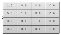
The main property of the identity matrix is that if it is multiplied by any other matrix, the values multiplied by zero do not change.
2.2 Transformation operations
Most transformations preserve the parallel relationship among the parts of the geometry. For example collinear points remain collinear after the transformation. Also points on one plane stay coplanar after transformation. This type of transformation is called an affine transformation.
Translation (move) transformation
Moving a point from a starting position by certain a vector can be calculated as follows:
$$P’ = P + \mathbf{\vec v}$$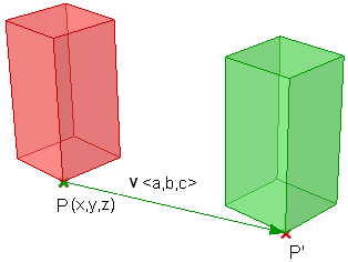
Suppose:
$$P(x,y,z)$$ is a given point
$$\mathbf{\vec v}=<a,b,c>$$ is a translation vector
Then:
$$P’(x) = x + a$$
$$P’(y) = y + b$$
$$P’(z) = z + c$$
Points are represented in a matrix format using a [4x1] matrix with a 1 inserted in the last row. For example the point P(x,y,z) is represented as follows:
$$\begin{bmatrix}x\\y\\z\\1\\\end{bmatrix}$$Using a $$[4 \times 4]$$ matrix for transformations (what is called a homogenous coordinate system), instead of a $$[3 \times 3]$$ matrices, allows representing all transformations including translation. The general format for a translation matrix is:
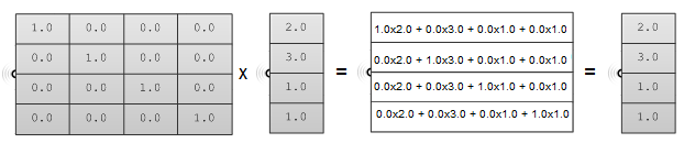
$$\begin{bmatrix}1 & 0 & 0 & \color{red}{a1} \\0 & 1 & 0 & \color{red}{a2} \\0 & 0 & 1 & \color{red}{a3} \\0 & 0 & 0 & 1 \\\end{bmatrix}$$For example, to move point $$P(2,3,1)$$ by vector $$\vec v <2,2,2>$$, the new point location is:
$$P’ = P + \mathbf{\vec v} = (2+2, 3+2, 1+2) = (4, 5, 3)$$If we use the matrix form and multiply the translation matrix by the input point, we get the new point location as in the following:
$$\begin{bmatrix}1 & 0 & 0 & 2 \\0 & 1 & 0 & 2 \\0 & 0 & 1 & 2 \\0 & 0 & 0 & 1 \\\end{bmatrix}\cdot\begin{bmatrix}2 \\3\\1\\1 \\\end{bmatrix}= \begin{bmatrix}(1*2 + 0*3 + 0*1 + 2*1) \\(0*2 + 1*3 + 0*1 + 2*1)\\(0*2 + 0*3 + 1*1 + 2*1)\\(0*2 + 0*3 + 0*1 + 1*1)\\\end{bmatrix}=\begin{bmatrix}4 \\5\\3\\1 \\\end{bmatrix}$$Similarly, any geometry is translated by multiplying its construction points by the translation matrix. For example, if we have a box that is defined by eight corner points, and we want to move it 4 units in the x-direction, 5 units in the y-direction and 3 units in the z- direction, we must multiply each of the eight box corner points by the following translation matrix to get the new box.
$$\begin{bmatrix}1 & 0 & 0 & 4\\ 0 & 1 & 0 & 5 \\0 & 0 & 1 & 3 \\0 & 0 & 0 & 1 \\\end{bmatrix}$$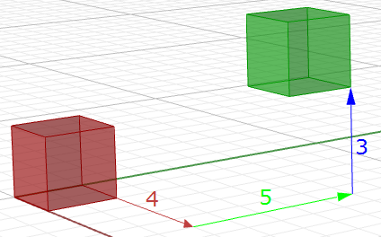
Rotation transformation
This section shows how to calculate rotation around the z-axis and the origin point using trigonometry, and then to deduce the general matrix format for the rotation.
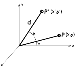
Take a point on $$x,y$$ plane $$P(x,y)$$ and rotate it by angle( $$b$$). From the figure, we can say the following:
$$x = d cos(a)$$ (1)
$$y = d sin(a)$$ (2)
$$x’ = d cos(b+a)$$ (3)
$$y’ = d sin(b+a)$$ (4)
Expanding
$$x$$’ and
$$y’$$ using trigonometric identities for the sine and cosine of the sum of angles:
$$x’ = d cos(a)cos(b) - d sin(a)sin(b)$$ (5)
$$y’ = d cos(a)sin(b) + d sin(a)cos(b)$$ (6)
Using Eq 1 and 2:
$$x’ = x cos(b) - y sin(b)$$
y’ = x sin(b) + y cos(b)
The rotation matrix around the z-axis looks like:
$$\begin{bmatrix}\color{red}{\cos{b}} & \color{red}{-\sin{b}} & 0 & 0 \\\color{red}{\sin{b}} & \color{red}{\cos{b}} & 0 & 0 \\0 & 0 & 1 & 0 \\0 & 0 & 0 & 1 \\\end{bmatrix}$$The rotation matrix around the x-axis by angle $$b$$ looks like:
$$\begin{bmatrix}1 & 0 & 0 & 0 \\0 & \color{red}{\cos{b}} & \color{red}{-\sin{b}} & 0 \\0 & \color{red}{\sin{b}} & \color{red}{\cos{b}} & 0 \\0 & 0 & 0 & 1 \\\end{bmatrix}$$The rotation matrix around the y-axis by angle $$b$$ looks like:
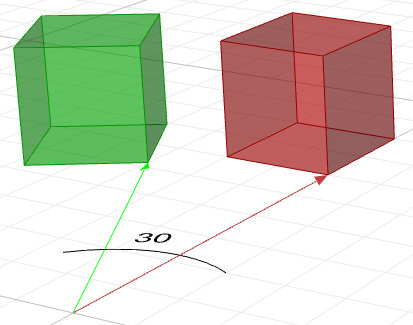
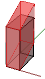
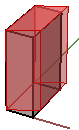
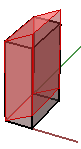
$$\begin{bmatrix}\color{red}{\cos{b}} &0 & \color{red}{\sin{b}} & 0 \\0 & 1 & 0 & 0 \\\color{red}{-\sin{b}} & 0 &\color{red}{\cos{b}} & 0 \\0 & 0 & 0 & 1 \\\end{bmatrix}$$For example, if we have a box and would like to rotate it 30 degrees, we need the following:
1. Construct the 30-degree rotation matrix. Using the generic form and the cos and sin values of 30-degree angle, the rotation matrix will look like the following:
$$\begin{bmatrix}0.87 & -0.5 & 0 & 0 \\0.5 & 0.87 & 0 & 0 \\0 & 0 & 1 & 0 \\0 & 0 & 0 & 1 \\\end{bmatrix}$$2. Multiply the rotation matrix by the input geometry, or in the case of a box, multiply by each of the corner points to find the box’s new location.
Scale transformation
In order to scale geometry, we need a scale factor and a center of scale. The scale factor can be uniform scaling equally in x-, y-, and z-directions, or can be unique for each dimension.
Scaling a point can use the following equation:
$$P’ = ScaleFactor(S) * P$$
Or:
$$P’.x = Sx * P.x$$
$$P’.y = Sy * P.y$$
$$P’.z = Sz * P.z$$
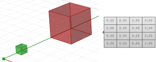
This is the matrix format for scale transformation, assuming that the center of scale is the World origin point (0,0,0).
$$\begin{bmatrix}\color{red}{Scale-x} & 0 & 0 & 0 \\0 & \color{red}{Scale-y} & 0 & 0 \\0 & 0 & \color{red}{Scale-z} & 0 \\0 & 0 & 0 & 1 \\\end{bmatrix}$$For example, if we would like to scale a box by 0.25 relative to the World origin, the scale matrix will look like the following:
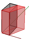
Shear transformation
Shear in 3‑D is measured along a pair of axes relative to a third axis. For example, a shear along a z‑axis will not change geometry along that axis, but will alter it along x and y. Here are few examples of shear matrices:
1. Shear in x and z, keeping the y-coordinate fixed:
 $$\begin{bmatrix}1.0 &\color{red}{0.5} & 0.0 & 0.0 \\ 0.0 & 1.0 & 0.0 & 0.0 \\ 0.0 & 0.0 & 1.0 & 0.0 \\ 0.0 & 0.0 & 0.0 & 1.0 \\\end{bmatrix}$$
 $$\begin{bmatrix}1.0 & 0.0 & 0.0 & 0.0 \\ 0.0 & 1.0 & 0.0 & 0.0 \\ 0.0 &\color{red}{0.5} & 1.0 & 0.0 \\ 0.0 & 0.0 & 0.0 & 1.0 \\\end{bmatrix}$$
2. Shear in y and z, keeping the x-coordinate fixed:
 $$\begin{bmatrix}1.0 & \color{red}{0.5} & 0.0 & 0.0 \\ 0.0 & 1.0 & 0.0 & 0.0 \\ 0.0 & 0.0 & 1.0 & 0.0 \\ 0.0 & 0.0 & 0.0 & 1.0 \\\end{bmatrix}$$
 $$\begin{bmatrix}1.0 & 0.0 & 0.0 & 0.0 \\ 0.0 & 1.0 & 0.0 & 0.0 \\ 0.0 & \color{red}{0.5} & 1.0 & 0.0 \\ 0.0 & 0.0 & 0.0 & 1.0 \\\end{bmatrix}$$
3. Shear in x and y, keeping the z-coordinate fixed:
 $$\begin{bmatrix}1.0 & 0.0 & \color{red}{0.5} & 0.0 \\ 0.0 & 1.0 & 0.0 & 0.0 \\ 0.0 & 0.0 & 1.0 & 0.0 \\ 0.0 & 0.0 & 0.0 & 1.0 \\\end{bmatrix}$$
 $$\begin{bmatrix}1.0 & 0.0 & 0.0 & 0.0 \\ 0.0 & 1.0 & \color{red}{0.5} & 0.0 \\ 0.0 & 0.0 & 1.0 & 0.0 \\ 0.0 & 0.0 & 0.0 & 1.0 \\\end{bmatrix}$$
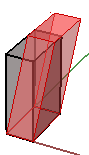
Mirror or reflection transformation
The mirror transformation creates a reflection of an object across a line or a plane. 2-D objects are mirrored across a line, while 3-D objects are mirrored across a plane. Keep in mind that the mirror transformation flips the normal direction of the geometry faces.
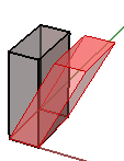
Planar Projection transformation
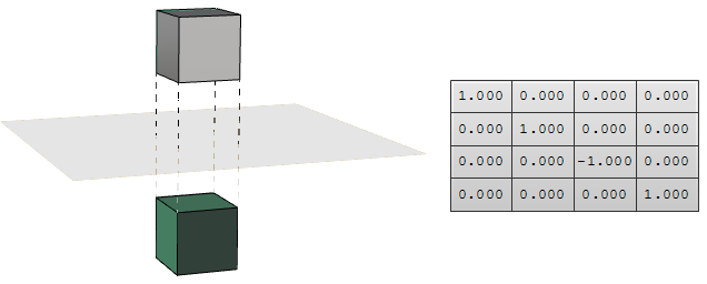
Intuitively, the projection point of a given 3-D point $$P(x,y,z)$$ on the world xy-plane equals $$P_{xy} (x,y,0)$$ setting the z value to zero. Similarly, a projection to xz-plane of point P is $$P_{xz}(x,0,z)$$. When projecting to yz-plane, $$P_{xz} = (0,y,z)$$. Those are called orthogonal projections.
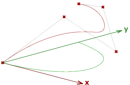
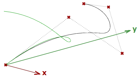
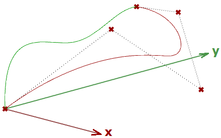
If we have a curve as an input, and we apply the planar projection transformation, we get a curve projected to that plane. The following shows an example of a curve projected to xy‑plane with the matrix format.
Note: NURBS curves (explained in the next chapter) use control points to define curves. Projecting a curve amounts to projecting its control points.
 $$\begin{bmatrix}1.0 & 0.0 & 0.0 & 0.0 \\ 0.0 & 1.0 & 0.0 & 0.0 \\ 0.0 & 0.0 & \color{red}{0.0} & 0.0 \\ 0.0 & 0.0 & 0.0 & 1.0 \\\end{bmatrix}$$
 $$\begin{bmatrix}1.0 & 0.0 & 0.0 & 0.0 \\ 0.0 & \color{red}{0.0} & 0.0 & 0.0 \\ 0.0 & 0.0 & 1.0 & 0.0 \\ 0.0 & 0.0 & 0.0 & 1.0 \\\end{bmatrix}$$
 $$\begin{bmatrix} \color{red}{0.0} & 0.0 & 0.0 & 0.0 \\ 0.0 & 1.0 & 0.0 & 0.0 \\ 0.0 & 0.0 & 1.0 & 0.0 \\ 0.0 & 0.0 & 0.0 & 1.0 \\\end{bmatrix}$$
Download Sample Files
Download the download samplesand tutorials archive, containing all the example Grasshopper and code files in this guide.
Next Steps
Now that you know more about matrices and trasnformasion, check out the Parametric Curves and Surfaces guide to learn more about the detailed structure of NURBS curves and surfaces.
