
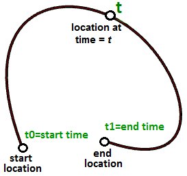
Suppose you travel every weekday from your house to your work. You leave at 8:00 in the morning and arrive at 9:00. At each point in time between 8:00 and 9:00, you would be at some location along the way. If you plot your location every minute during your trip, you can define the path between home and work by connecting the 60 points you plotted. Assuming you travel the exact same speed every day, at 8:00 you would be at home (start location), at 9:00 you would be at work (end location) and at 8:40 you would at the exact same location on the path as the 40th plot point. Congratulations, you have just defined your first parametric curve! You have used time as a parameter to define your path, and hence you can call your path curve a parametric curve. The time interval you spend from start to end (8 to 9) is called the curve domain or interval.
In general, we can describe the
$$x$$,
$$y$$, and
$$z$$ location of a parametric curve in terms of some parameter
$$t$$ as follows:
$$x = x(t)$$
$$y = y(t)$$
$$z = z(t)$$
Where:
$$t$$ is a range of real numbers
We saw earlier that the parametric equation of a line in terms of parameter $$t$$ is defined as:
$$x = x’ + t * a$$
$$y = y’ + t * b$$
$$z = z’ + t * c$$
Where:
$$x$$, $$y$$, and $$z$$ are functions of t where t represents a range of real numbers. $$x’$$, $$y’$$, and $$z’$$ are the coordinates of a point on the line segment. $$a$$, $$b$$, and $$c$$ define the slope of the line, such that the vector $$\mathbf{\vec v} <a, b, c>$$ is parallel to the line.
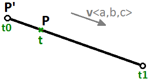
We can therefore write the parametric equation of a line segment using a $$t$$ parameter that ranges between two real number values $$t0$$, $$t1$$ and a unit vector $$\mathbf{\vec v}$$ that is in the direction of the line as follows:
$$P = P’ + t * \mathbf{\vec v}$$Another example is a circle. The parametric equation of the circle on the xy-plane with a center at the origin (0,0) and an angle parameter $$t$$ ranging between $$0$$ and $$2π$$ radians is:
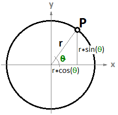
$$x = r \dot cos(t)$$
$$y = r \dot sin(t)$$
We can derive the general equation of a circle for the parametric one as follows:
$$ x/r = cos(t)$$
$$y/r = sin(t)$$
And since:
$$cos(t)^2 + sin(t)^2 = 1$$ (Pythagorean identity)
Then:
$$(x/r)^2 + (y/r)^2 = 1$$ , or
$$x^2 + y^2 = r^2$$
3.1 Parametric curves
Curve parameter
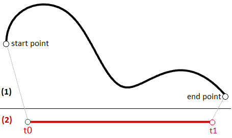
A parameter on a curve represents the address of a point on that curve. As mentioned before, you can think of a parametric curve as a path traveled between two points in a certain amount of time, traveling at a fixed or variable speed. If traveling takes $$T$$ amount of time, then the parameter t represents a time within $$T$$ that translates to a location (point) on the curve.
If you have a straight path (line segment) between the two points $$A$$ and $$B$$, and $$\mathbf{\vec v}$$ were a vector from $$A$$ to $$B$$ ( $$\mathbf{\vec v} = B - A$$), then you can use the parametric line equation to find all points $$M$$ between $$A$$ and $$B$$ as follows:
$$M = A + t*(B-A)$$
Where:
$$t$$ is a value between 0 and 1.
The range of t values, 0 to 1 in this case, is referred to as the curve domain or interval. If t was a value outside the domain (less that 0 or more than 1), then the resulting point $$M$$ will be outside the linear curve $$\overline{AB}$$.
The same principle applies for any parametric curve. Any point on the curve can be calculated using the parameter t within the interval or domain of values that define the limits of the curve. The start parameter of the domain is usually referred to as $$t0$$ and the end of the domain as $$t1$$.
Curve domain or interval
A curve domain or interval is defined as the range of parameters that evaluate into a point within that curve. The domain is usually described with two real numbers defining the domain limits expressed in the form (min to max)or (min, max). The domain limits can be any two values that may or may not be related to the actual length of the curve. In an increasing domain, the domain min parameter evaluates to the start point of the curve and the domain max evaluates to the end point ofthe curve.
Changing a curve domain is referred to as the process of reparameterizing the curve. For example, it is very common to change the domain to be (0 to 1). Reparameterizing a curve does not affect the shape of the 3-D curve. It is like changing the travel time on a path by running instead of walking, which does not change the shape of the path.
An increasing domain means that the minimum value of the domain points to the start of the curve. Domains are typically increasing, but not always.
Curve evaluation
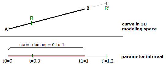
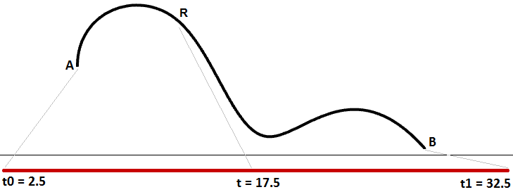
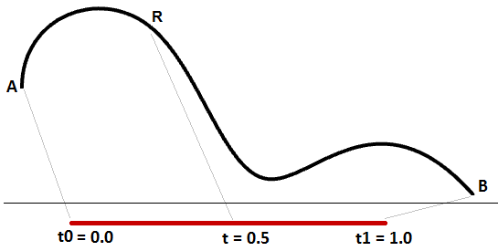
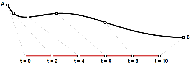
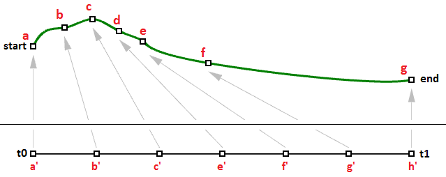
We learned that a curve interval is the range of all parameter values that evaluate to points within the 3-D curve. There is, however, no guarantee that evaluating at the middle of the domain, for example, will give a point that is in the middle of the curve, as shown in Figure (29).
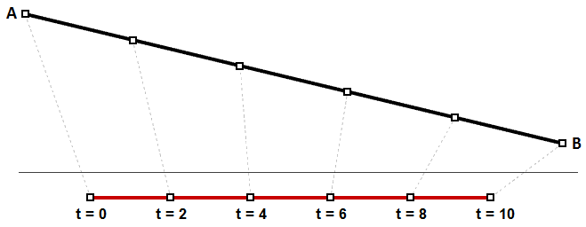
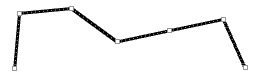
We can think of uniform parameterization of a curve as traveling a path with constant speed. A degree-1 line between two points is one example where equal intervals or parameters translate into equal intervals of arc length on the line. This is a special case where equal intervals of parameters evaluate to equal intervals on the 3-D curve.
It is, however, more likely that the speed decreases or increases along the path. For example, if it takes 30 minutes to travel a road, it is unlikely that you will be exactly half way through at minute 15. Figure (30) shows a typical case where equal parameter intervals evaluate to variable length on the 3-D curve.
You may need to evaluate points on a 3-D curve that are at a defined percentage of the curve length. For example, you might need to divide the curve into equal lengths. Typically, 3-D modelers provide tools to evaluate curves relative to arc length.
Tangent vector to a curve
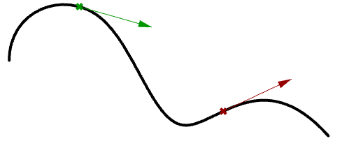
A tangent to a curve at any parameter (or point on a curve) is the vector that touches the curve at that point, but does not cross over. The slope of the tangent vector equals the slope of the curve at the same point. The following example evaluates the tangent to a curve at two different parameters.
Cubic polynomial curves
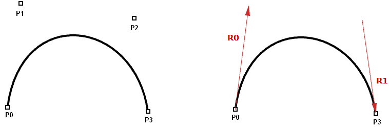
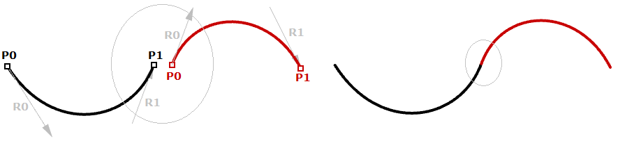
Hermite and Bézier curves are two examples of cubic polynomial curves that are determined by four parameters. A Hermite curve is determined by two end points and two tangent vectors at these points, while a Bézier curve is defined by four points. While they differ mathematically, they share similar characteristics and limitations.
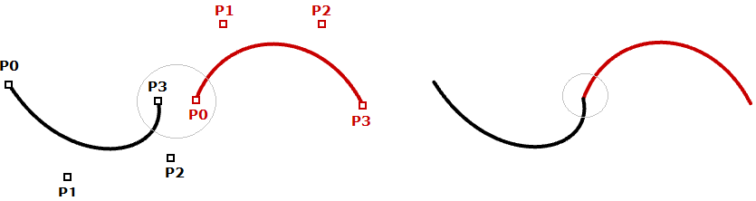
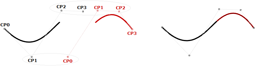
In most cases, curves are made out of multiple segments. This requires making what is called a piecewise cubic curve. Here is an illustration of a piecewise Bézier curve that uses 7 storage points to create a two-segment cubic curve. Note that although the final curve is joined, it does not look smooth or continuous.
Although Hermite curves use the same number of parameters as Bézier curves (four parameters to define one curve), they offer the additional information of the tangent curve that can also be shared with the next piece to create a smoother looking curve with less total storage, as shown in the following.
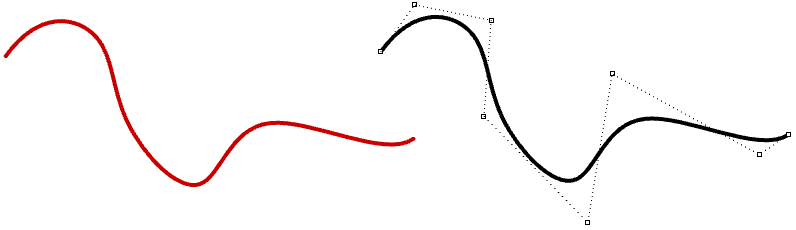
The non-uniform rational B-spline (NURBS) is a powerful curve representation that maintains even smoother and more continuous curves. Segments share more control points to achieve even smoother curves with less storage.
NURBS curves and surfaces are the main mathematical representation used by Rhino to represent geometry. NURBS curve characteristics and components will be covered with some detail later in this chapter.
Evaluating cubic Bézier curves
Named after its inventor, Paul de Casteljau, the de Casteljau algorithm evaluates Bézier curves using a recursive method. The algorithm steps can be summarized as follows:
Input:
Four points $$A$$, $$B$$, $$C$$, $$D$$ define a curve $$t$$, is any parameter within curve domain
Output:
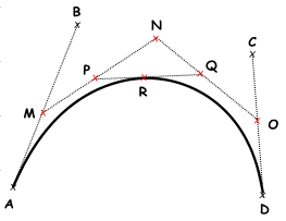
Point $$R$$ on curve that is at parameter $$t$$.
Solution:
- Find point
$$M$$ at
$$t$$ parameter on line
$$\overline{AB}$$.
2.Find point $$N$$ at $$t$$ parameter on line $$\overline{BC}$$.
3.Find point $$O$$ at $$t$$ parameter on line $$\overline{CD}$$.
4.Find point $$P$$ at $$t$$ parameter on line $$\overline{MN}$$.
5.Find point $$Q$$ at $$t$$ parameter on line $$\overline{NO}$$.
6.Find point $$R$$ at $$t$$ parameter on line $$\overline{PQ}$$.
3.2 NURBS curves
NURBS is an accurate mathematical representation of curves that is highly intuitive to edit. It is easy to represent free-form curves using NURBS and the control structure makes it easy and predictable to edit.
There are many books and references for those of you interested in an in-depth reading about NURBS. A basic understanding of NURBS is however necessary to help use a NURBS modeler more effectively. There are four main attributes define the NURBS curve: degree, control points, knots, and evaluation rules.
Degree
Curve degree is a whole positive number. Rhino allows working with any degree curve starting with 1. Degrees 1, 2, 3, and 5 are the most useful but the degrees 4 and those above 5 are not used much in the real world. Following are a few examples of curves and their degree:
| Lines and polylines are degree-1 NURBS curves. | 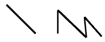 |
| Circles and ellipses are examples of degree-2 NURBS curves. | 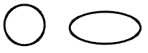 |
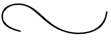
| Free-form curves are usually represented as degree-3 or 5 NURBS curves. |
 |
Control points
The control points of a NURBS curve is a list of at least (degree+1) points. The most intuitive way to change the shape of a NURBS curve is through moving its control points.
The number of control points that affect each span in a NURBS curve is defined by the degree of the curve. For example, each span in a degree-1 curve is affected only by the two end control points. In a degree-2 curve, three control points affect each span and so on.
| Control points of degree-1 curves go through all curve control points. In a degree-1 NURBS curve, two (degree+1) control points define each span. Using five control points, the curve has four spans. | 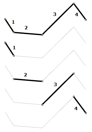 |
| Circles and ellipses are examples of degree two curves. In a degree-2 NURBS curve, three (degree+1) control points define each span. Using five control points, the curve has three spans. | 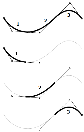 |
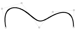
| Control points of degree‑3 curves do not usually touch the curve, except at the end points in open curves. In a degree‑3 NURBS curve, four (degree+1) control points define each span. Using five control points, the curve has two spans | 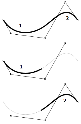 |
Weights of control points
Each control point has an associated number called weight. With a few exceptions, weights are positive numbers. When all control points have the same weight, usually 1, the curve is called non-rational. Intuitively, you can think of weights as the amount of gravity each control point has. The higher the relative weight a control point has, the closer the curve is pulled towards that control point.
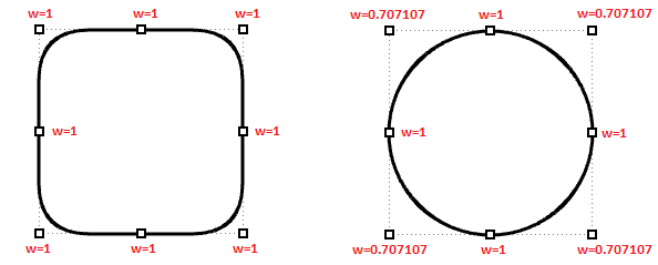
It is worth noting that it is best to avoid changing curve weights. Changing weights rarely gives desired result while it introduces a lot of calculation challenges in operations such as intersections. The only good reason for using rational curves is to represent curves that cannot otherwise be drawn, such as circles and ellipses.
Knots
Each NURBS curve has a list of numbers associated with it called a list of knots (sometimes referred to as knot vector). Knots are a little harder to understand and set. While using a 3-D modeler, you will not need to manually set the knots for each curve you create; a few things will be useful to learn about knots.
Knots are parameter values
Knots are a non-decreasing list of parameter values that lie within the curve domain. In Rhino, there is degree-1 more knots than control points. That is the number of knots equals the number of control points plus curve degree minus 1:
|knots| = |CVs| + Degree - 1
Usually, for non-periodic curves, the first degree many knots are equal to the domain minimum, and the last degree many knots are equal to the domain maximum.
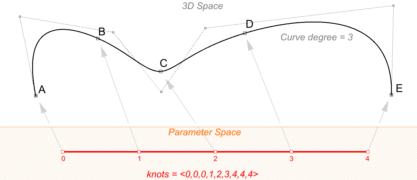
For example, the knots of an open degree-3 NURBS curve with 7 control points and a domain between 0 and 4 may look like <0, 0, 0, 1, 2, 3, 4, 4, 4>.
Scaling a knot list does not affect the 3D curve. If you change the domain of the curve in the above example from “0 to 4” to “0 to 1”, knot list get scaled, but the 3D curve does not change.
We call a knot with value appearing only once as simple knot. Interior knots are typically simple as in the two examples above.
Knot multiplicity
The multiplicity of a knot is the number of times it is listed in the list of knots. The multiplicity of a knot cannot be more than the degree of the curve. Knot multiplicity is used to control continuity at the corresponding curve point.
Fully-multiple knots
A fully multiple knot has multiplicity equal to the curve degree. At a fully multiple knot there is a corresponding control point, and the curve goes through this point.
For example, clamped or open curves have knots with full multiplicity at the ends of the curve. This is why the end control points coincide with the curve end points. Interior fully multiple knots allow a kink in the curve at the corresponding point.
For example, the following two curves are both degree-3, and have the same number and location of control points. However they have different knots and their shape is also different. Fully multiplicity forces the curve through the associated control point.
Here are two curves that have the same degree, and same number and location of control points, and yet have different knots vector that results in different curve shape:
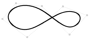
| Degree = 3 Number of control points = 7 knots = <0,0,0,1,2,3,4,4,4> = 9 knots Domain (0 to 4) |
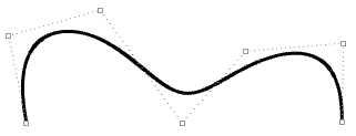 |
| Degree = 3 Number of control points = 7 knots = <0,0,0,1,1,1,4,4,4> = 9 knots Domain (0 to 4) Note: A fully multiple knot in the middle creates a kink and the curve is forced to go through the associated control point. |
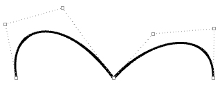 |
Uniform knots
A uniform list of knots satisfies the following condition.
Knots start with a fully-multiple knot, are followed by simple knots, and terminate with a fully-multiple knot. The values are increasing and equally spaced. This is typical of clamped or open curves. Periodic curves work differently as we will see later.
Non uniform knots
NURBS curves are allowed to have non-uniform spacing between knots. This can help control the curvature along the curve to create more smooth curves. Take the following example interpolating through points using non-uniform knots list in the left, and uniform in the right. In general, if a NURBS curve spacing of knots is proportional to the spacing between control points, then the curve is smoother.
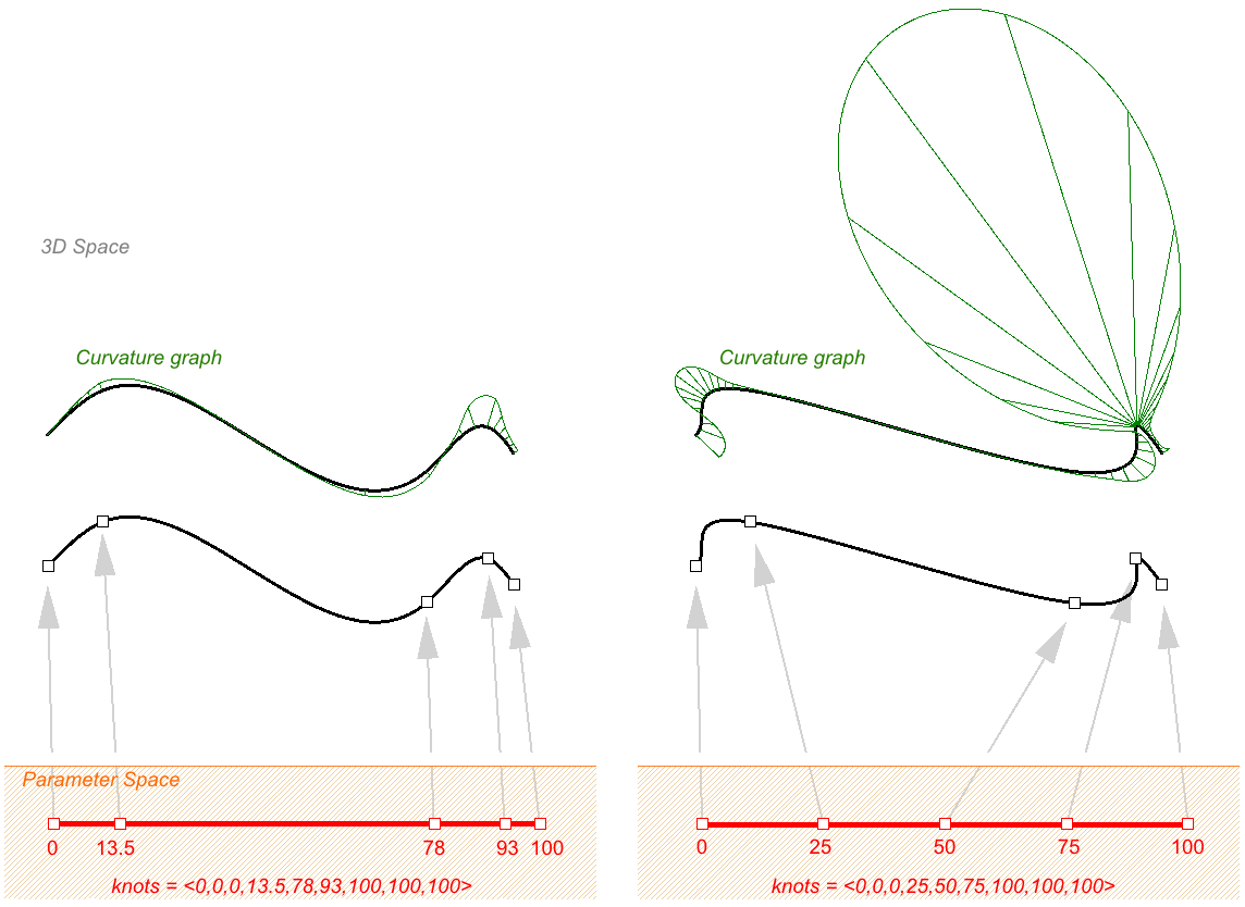
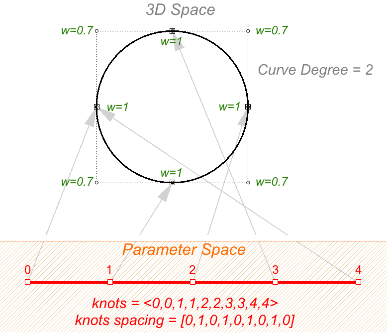
An example of a curve that is both non-uniform and rational is a NURBS circle. The following is a degree 2 curve with 9 control points and 10 knots. Domain is 0-4, and the spacing alternate between 0 and 1. knots = <0,0,1,1,2,2,3,3,4,4> — (full multiplicity in the interior knots) spacing between knots = [0,1,0,1,0,1,0,1,0] — (non-uniform)
Evaluation rule
The evaluation rule uses a mathematical formula that takes a number within the curve domain and assigns a point. The formula takes into account the degree, control points, and knots.
Using this formula, specialized curve functions can take a curve parameter and produce the corresponding point on that curve. A parameter is a number that lies within the curve domain. Domains are usually increasing and consist of two numbers: the minimum domain parameter $$t(0)$$ that evaluates to the start point of the curve and the maximum $$t(1)$$ that evaluates to the end point of the curve.
Characteristics of NURBS curves
In order tocreate a NURBS curve, you will need to provide the followinginformation:
- Dimension, typically 3
- Degree, (sometimes use the order,which is equal to degree+1)
- Control points (list of points)
- Weight of the control point (listof numbers)
- Knots (list of numbers)
When you create a curve, you need to at least define the degree and locations of the control points. The rest of the information necessary to construct NURBS curves can be generated automatically. Selecting an end point to coincide with the start point would typically create a periodic smooth closed curve. The following table shows examples of open and closed curves:
| Degree-1 open curve. The curve goes through all control points. |
 |
| Degree-3 open curve. Both curve ends coincide with end control points. |
 |
| Degree-3 closed periodic curve. The curve seam does not go through a control point. |
 |
| Moving control points of a periodic curve does not affect curve smoothness. | 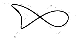 |
| Kinks are created when the curve is forced through some control points. | 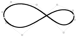 |
| Moving the control points of a non-periodic curve does not guarantee smooth continuity of the curve, but enables more control over the outcome. | 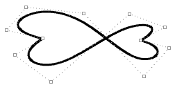 |
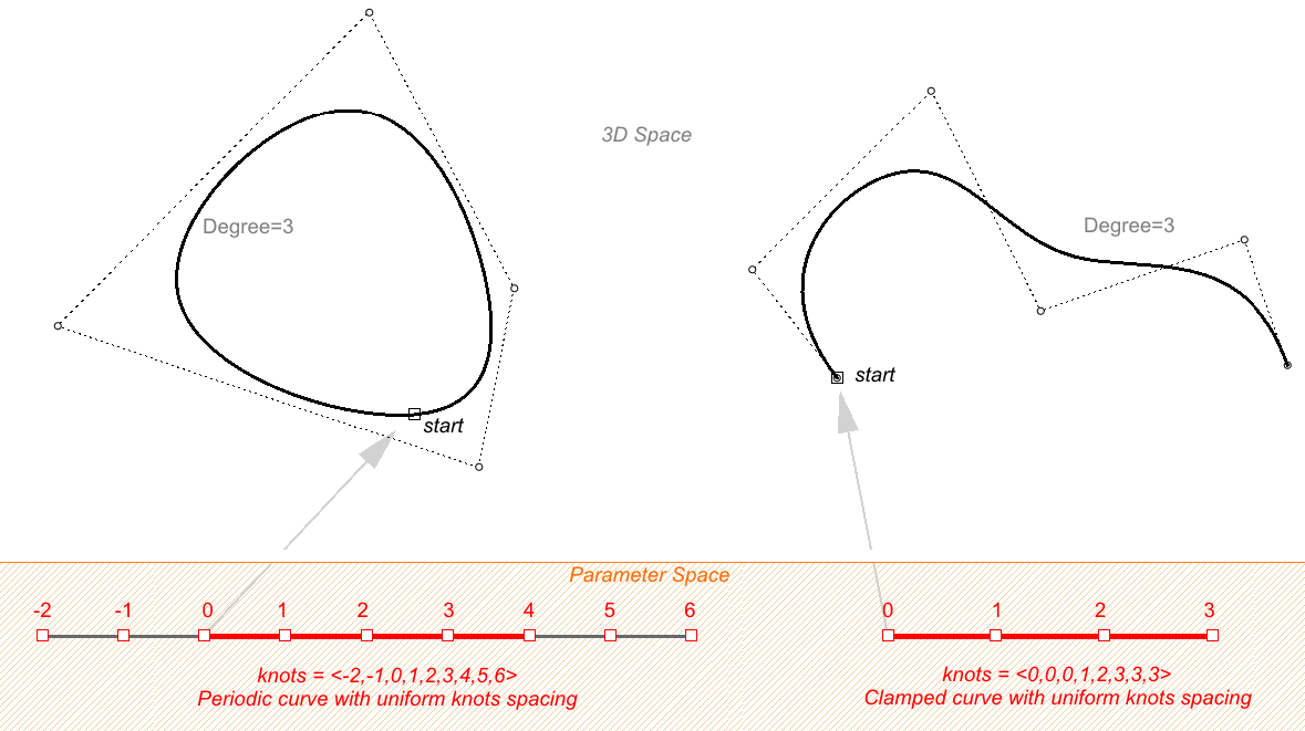
Clamped vs. periodic NURBS curves
The end points of closed clamped curves coincide with end control points. Periodic curves are smooth closed curves. The best way to understand the differences between the two is through comparing control points and knots.
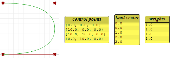
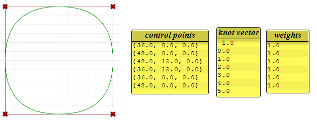
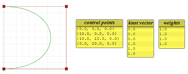
The following is an example of an open, clamped non-rational NURBS curve. This curve has four control points, uniform knots with full-multiplicity at the start and end knots and the weights of all control points equal to 1.
The following circular curve is an example of a degree-3 closed periodic NURBS curve. It is also non-rational because all weights are equal. Note that periodic curves require more control points with few overlapping. Also the knots are simple.
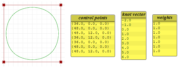
Notice that the periodic curve turned the four input points into seven control points (degree+4), while the clamped curve used only the four control points. The knots of the periodic curve uses only simple knots, while the clamped curve start and end knots have full multiplicity forcing the curve to go through the start and end control points.
If we set the degree of the previous examples to 2 instead of 3, the knots become smaller, and the number of control points of periodic curves changes.
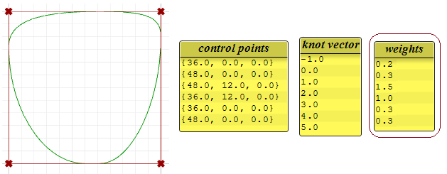
Weights
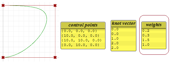
Weights of control points in a uniform NURBS curve are set to 1, but this number can vary in rational NURBS curves. The following example shows the effect of varying the weights of control points.
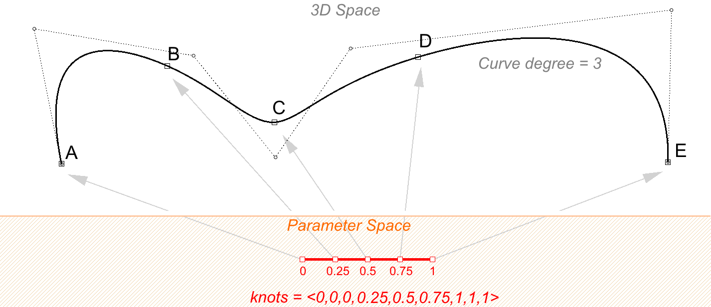
Evaluating NURBS curves
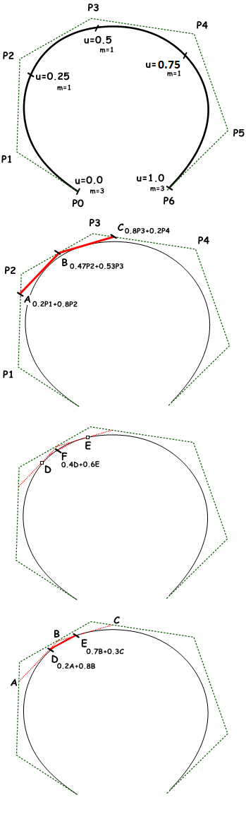
Named after its inventor, Carl de Boor, the de Boor’s algorithmi is a generalization of the de Casteljau algorithm for Bézier curves. It is numerically stable and is widely used to evaluate points on NURBS curves in 3-D applications. The following is an example for evaluating a point on a degree-3 NURBS curve using de Boor’s algorithm.
Input:
Seven control points
$$P0$$ to
$$P6$$
Knots:
$$u_0 = 0.0$$
$$u_1 = 0.0$$
$$u_2 = 0.0$$
$$u_3= 0.25$$
$$u_4 = 0.5$$
$$u_5 = 0.75$$
$$u_6 = 1.0$$
$$u_7 = 1.0$$
$$u_8 = 1.0$$
Output:
Point on curve that is at $$u=0.4$$
Solution:
1. Calculate coefficients for the first iteration:
$$A_c = ((u – u_1)/(u_{1+3} – u_1) = 0.8$$
$$B_c = (u – u_2)/(u_{2+3} – u_2) = 0.53$$
$$C_c = (u – u_3)/(u_{3+3} – u_3) = 0.2$$
2. Calculate points using coefficient data:
$$A = 0.2P_1 + 0.8P_2$$
$$B = 0.47 P_2 + 0.53 P_3$$
$$C = 0.8 P_3 + 0.2 P_4$$
3. Calculate coefficients for the second iteration:
$$D_c = (u – u_2) / (u_{2+3-1} – u_2) = 0.8$$
$$E_c = (u – u_3) / (u_{3+3-1} – u_3) = 0.3$$
4. Calculate points using coefficient data:
$$D = 0.2A+ 0.8B$$
$$E = 0.7B + 0.3C$$
5. Calculate the last coefficient:
$$Fc = (u – u_3)/ (u_{3+3-2} – u_3) = 0.6$$
Find the point on curve at $$u=0.4$$ parameter:
$$F= 0.4D + 0.6E$$
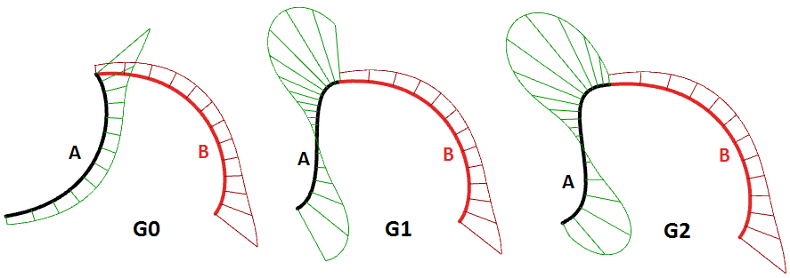
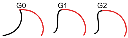
3.3 Curve geometric continuity
Continuity is an important concept in 3‑D modeling. Continuity is important for achieving visual smoothness and for obtaining smooth light and airflow. The following table shows various continuities and their definitions:
| G0| (Position continuous) | Two curve segments joined together |
| G1| (Tangent continuous) | Direction of tangent at joint point is the same for both curve segments. |
| G2| ( Curvature Continuous) | Curvatures as well as tangents agree for both curve segments at the common endpoint. |
| GN|……. | The curves agree to higher order |
3.4 Curve curvature
Curvature is a widely used concept in modeling 3‑D curves and surfaces. Curvature is defined as the change in inclination of a tangent to a curve over unit length of arc. For a circle or sphere, it is the reciprocal of the radius and it is constant across the full domain.
At any point on a curve in the plane, the line best approximating the curve that passes through this point is the tangent line. We can also find the best approximating circle that passes through this point and is tangent to the curve. The reciprocal of the radius of this circle is the curvature of the curve at this point.
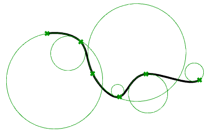
The best approximating circle can lie either to the left or to the right of the curve. If we care about this, we establish a convention, such as giving the curvature positive sign if the circle lies to the left and negative sign if the circle lies to the right of the curve. This is known as signed curvature. Curvature values of joined curves indicate continuity between these curves.
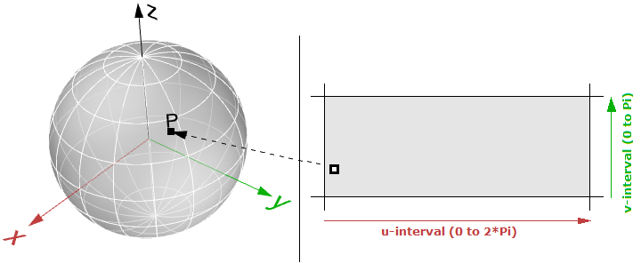
3.5 Parametric surfaces
Surface parameters
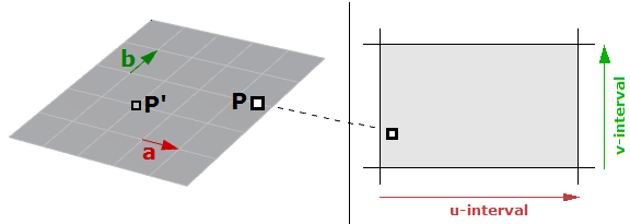
A parametric surface is a function of two independent parameters (usually denoted $$u$$, $$v$$) over some two-dimensional domain. Take for example a plane. If we have a point $$P$$ on the plane and two nonparallel vectors on the plane, $$\vec a$$ and $$\vec b$$, then we can define a parametric equation of the plane in terms of the two parameters $$u$$ and $$v$$ as follows:
$$P = P’ + u * \mathbf{\vec a} + v * \mathbf{\vec b}$$Where:
$$P’$$: is a known point on the plane
$$\mathbf{\vec a}$$: is the first vector on the plane
$$\mathbf{\vec b}$$: is the first vector on the plane
$$u$$: is the first parameter
$$v$$: is the first parameter
Another example is the sphere. The Cartesian equation of a sphere centered at the origin with radius $$R$$ is
$$x^2 + y^2 + z^2 = R^2$$That means for each point, there are three variables ( $$x$$, $$y$$, $$z$$), which is not useful to use for a parametric representation that requires only two variables. However, in the spherical coordinate system, each point is found using the three values:
$$r$$: radial distance between the point and the origin
$$θ$$: the angle from the x-axis in the xy-plane
$$ø$$: the angle from the z-axis and the point
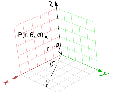
A conversion of points from spherical to Cartesian coordinate can be obtained as follows:
$$x = r * sin(ø) * cos(θ)$$
$$y = r * sin(ø) * sin(θ)$$
$$z = r * cos (ø)$$
Where:
$$r$$ is distance from origin
$$≥ 0$$
$$θ$$ is running from
$$0$$ to
$$2π$$
$$ø$$ is running from
$$0$$ to
$$π$$
Since $$r$$ is constant in a sphere surface, we are left with only two variables, and hence we can use the above to create a parametric representation of a sphere surface:
$$u = θ$$
$$v = ø$$
So that:
$$x = r * sin(v) * cos(u)$$
$$y = r * sin(v) * sin(u)$$
$$z = r * cos(v)$$
Where ( $$u$$, $$v$$) is within the domain ( $$2 π$$, $$π$$)
The parametric surface follows the general form:
$$x = x(u,v)$$
$$y = y(u,v)$$
$$z = z(u,v)$$
Where:
$$u$$ and $$v$$ are the two parameters within the surface domain or region.
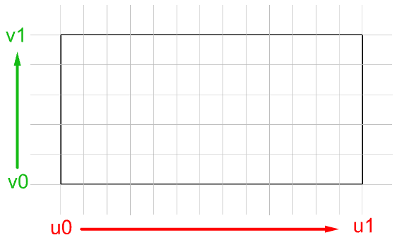
Surface domain
A surface domain is defined as therange of ( $$u,v$$) parameters that evaluate into a 3 D point on thatsurface. The domain in each dimension ( $$u$$ or $$v$$) is usually describedas two real numbers ( $$u_{min}$$ to $$u_{max}$$) and ( $$v_{min}$$ to $$v_{max}$$)
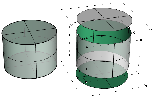
Changing a surface domain is referredto as reparameterizing the surface. An increasingdomain means that the minimum value of the domain points to theminimum point of the surface. Domains are typically increasing, butnot always.
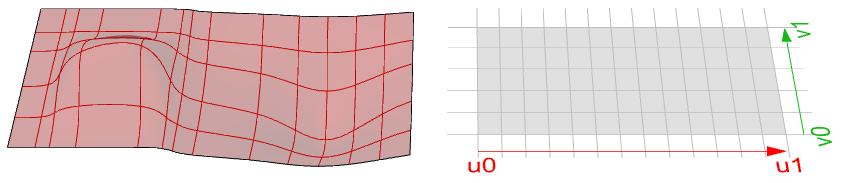
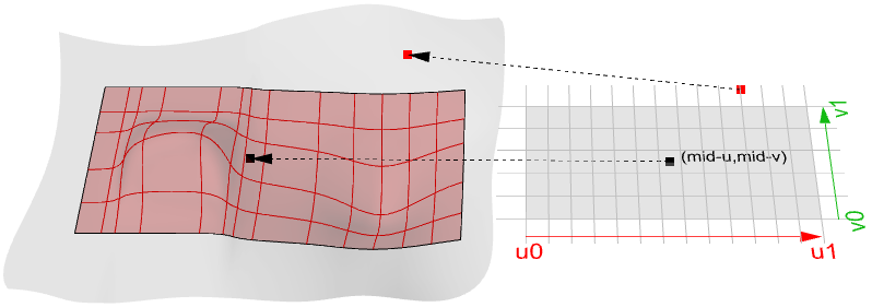
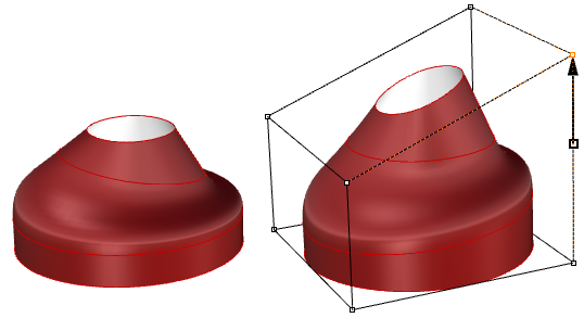
Surface evaluation
Evaluating a surface at a parameter that is within the surface domain results in a point that is on the surface. Keep in mind that the middle of the domain ( $$u_{mid}$$, $$v_{mid}$$) might not necessarily evaluate to the middle point of the 3-D surface. Also, evaluating $$u-$$ and $$v-$$ values that are outside the surface domain will not give a useful result.
Tangent plane of a surface
The tangent plane to a surface at a given point is the plane that touches the surface at that point. The z-direction of the tangent plane represents the normal direction of the surface at that point.

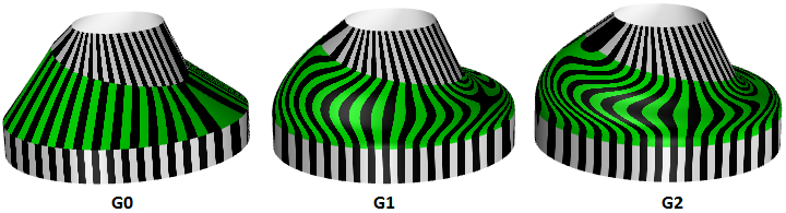
3.6 Surface geometric continuity
Many models cannot be constructed from one surface patch. Continuity between joined surface patches is important for visual smoothness, light reflection, and airflow. The following table shows various continuities and their definitions:
| G0 | (Position continuous) | Two surfaces joined together. |
| G1 | (Tangent continuous) | The corresponding tangents of the two surfaces along their joint edge are parallel in both u‑ and v‑directions. |
| G2 | ( Curvature Continuous) | Curvatures as well as tangents agree for both surfaces at the common edge. |
| GN | ……. | The surfaces agree to higher order. |
3.7 Surface curvature
For surfaces, normal curvature is one generalization of curvature to surfaces. Given a point on the surface and a direction lying in the tangent plane of the surface at that point, the normal section curvature is computed by intersecting the surface with the plane spanned by the point, the normal to the surface at that point, and the direction. The normal section curvature is the signed curvature of this curve at the point of interest.
If we look at all directions in the tangent plane to the surface at our point, and we compute the normal curvature in all these directions, there will be a maximum value and a minimum value.
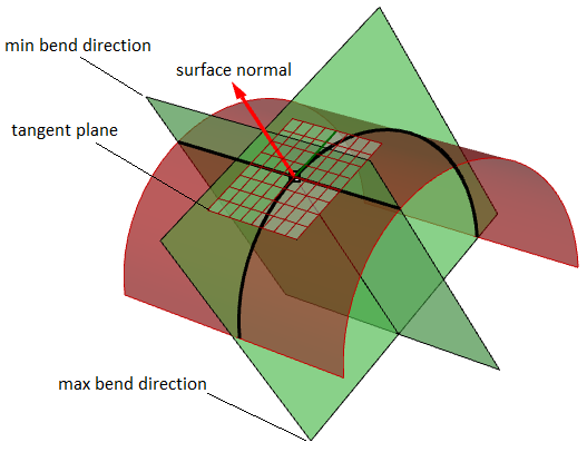
Principal curvatures
The principal curvatures of a surface at a point are the minimum and maximum of the normal curvatures at that point. They measure the maximum and minimum bend amount of the surface at that point. The principal curvatures are used to compute the Gaussian and mean curvatures of the surface.
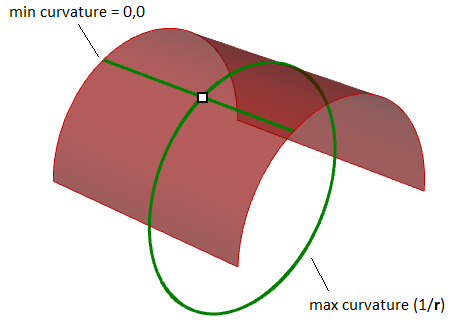
For example, in a cylindrical surface, there is no bend along the linear direction (curvature equals zero) while the maximum bend is when intersecting with a plane parallel to the end faces (curvature equals 1/radius). Those two extremes make the principle curvatures of that surface.
Gaussian curvature
The Gaussian curvature of a surface at a point is the product of the principal curvatures at that point. The tangent plane of any point with positive Gaussian curvature touches the surface locally at a single point, whereas the tangent plane of any point with negative Gaussian curvature cuts the surface.
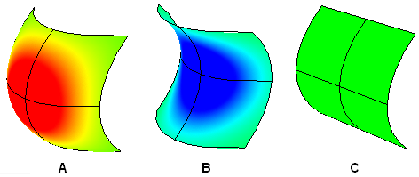
A: Positive curvature when surface is bowl-like.
B: Negative curvature when surface is saddle-like.
C: Zero curvature when surface is flat in at least one direction (plane, cylinder).
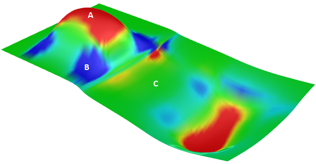
Mean curvature
The mean curvature of a surface at a point is one-half of the sums of the principal curvatures at that point. Any point with zero mean curvature has negative or zero Gaussian curvature.
Surfaces with zero mean curvature everywhere are minimal surfaces. Physical processes which can be modeled by minimal surfaces include the formation of soap films spanning fixed objects, such as wire loops. A soap film is not distorted by air pressure (which is equal on both sides) and is free to minimize its area. This contrasts with a soap bubble, which encloses a fixed quantity of air and has unequal pressures on its inside and outside. Mean curvature is useful for finding areas of abrupt change in the surface curvature.
Surfaces with constant mean curvature everywhere are often referred to as constant mean curvature (CMC) surfaces. CMC surfaces include the formation of soap bubbles, both free and attached to objects. A soap bubble, unlike a simple soap film, encloses a volume and exists in equilibrium where slightly greater pressure inside the bubble is balanced by the area-minimizing forces of the bubble itself.
3.8 NURBS surfaces
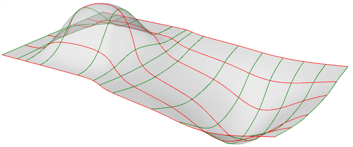
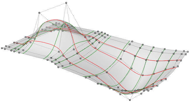
You can think of NURBS surfaces as a grid of NURBS curves that go in two directions. The shape of a NURBS surface is defined by a number of control points and the degree of that surface in each one of the two directions (u- and v-directions). NURBS surfaces are efficient for storing and representing free-form surfaces with a high degree of accuracy. The mathematical equations and details of NURBS surfaces are beyond the scope of this text. We will only focus on the characteristics that are most useful for designers.
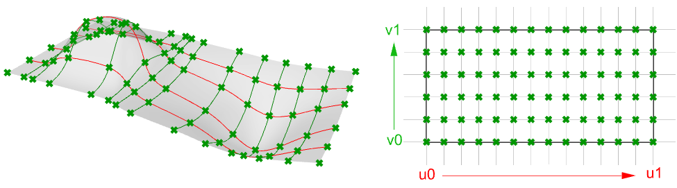
Evaluating parameters at equal intervals in the 2-D parameter rectangle does not translate into equal intervals in 3-D space in most cases.
Characteristics of NURBS surfaces
NURBS surface characteristics are very similar to NURBS curves except there is one additional parameter. NURBS surfaces hold the following information:
- Dimension, typically 3
- Degree in u‑and v‑directions: (sometimes use order which is degree + 1)
- Control points (points)
- Weights of control points (numbers)
- Knots (numbers)
As with the NURBS curves, you will probably not need to know the details of how to create a NURBS surface, since 3-D modelers will typically provide good set of tools for this. You can always rebuild surfaces (and curves for that matter) to a new degree and number of control points. Surface can be open, closed, or periodic. Here are few examples of surfaces:
| Degree-1 surface in both u- and v-directions. All control points lie on the surface. | 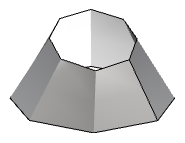 |
| Degree-3 in the u-direction and degree‑1 in the v-direction open surface. The surface corners coincide with corner control points. | 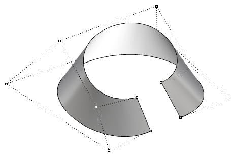 |
| Degree-3 in the u-direction and degree 1 in the v-direction closed (non-periodic) surface. Some control points coincide with the surface seam. | 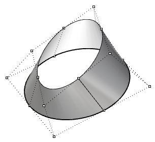 |
| Moving control points of a closed (non-periodic) surface causes a kink and the surface does not look smooth. | 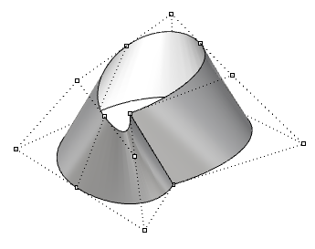 |
| Degree 3 the u-direction and degree 1 in the v-direction periodic surface. The surface control points do not coincide with the surface seam. | 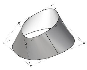 |
| Moving the control points of a periodic surface does not affect surface smoothness or create kinks. | 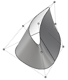 |
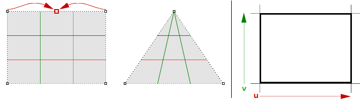
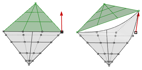
Singularity in NURBS surfaces
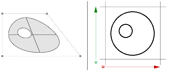
For example, if you have a linear edge of a simple plane, and you drag the two end control points of an edge so they overlap (collapse) at the middle, you will get a singular edge. You will notice that the surface isocurves converge at the singular point.
The above triangular shape can be created without singularity. You can trim a surface with a triangle polyline. When you examine the underlying NURBS structure, you see that it remains a rectangular shape.
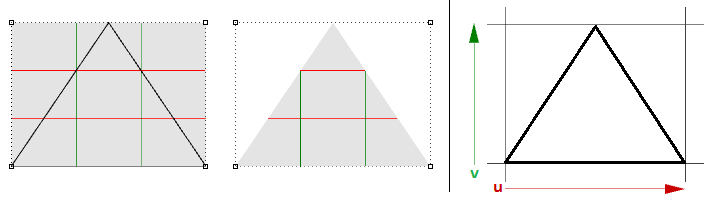
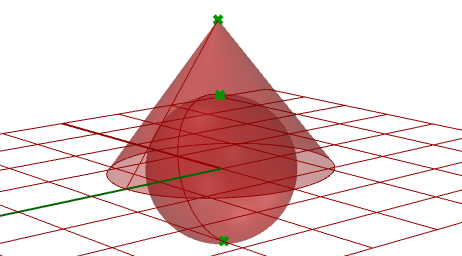
Other common examples of surfaces that are hard to generate without singularity are the cone and the sphere. The top of a cone and top and bottom edges of a sphere are collapsed into one point. Whether there is singularity or not, the parameter rectangle maintains a more or less rectangular region.
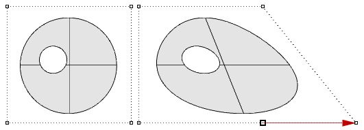
Trimmed NURBS surfaces
NURBS surfaces can be trimmed or untrimmed. Trimmed surfaces use an underlying NURBS surface and closed curves to trim out part of that surface. Each surface has one closed curve that defines the outer border (outer loop) and can have non-intersecting closed inner curves to define holes (inner loops). A surface with an outer loop that is the same as that of its underlying NURBS surface and that has no holes is what we refer to as an untrimmed surface.
3.9 Polysurfaces
A polysurface consists of two or more(possibly trimmed) NURBS surfaces joined together. Each surface hasits own structure, parameterization, and isocurve directions that donot have to match. Polysurfaces are represented using the boundaryrepresentation (BRep). The BRep structure describes surfaces,edges, and vertices with trimming data and connectivity amongdifferent parts. Trimmed surface are also represented using BRep datastructure.
The BRep is a data structure that describes each face in terms of its underlying surface, surrounding 3-D edges, vertices, parameter space 2-D trims, and relationship between neighboring faces. BRep objects are also called solids when they are closed (watertight).
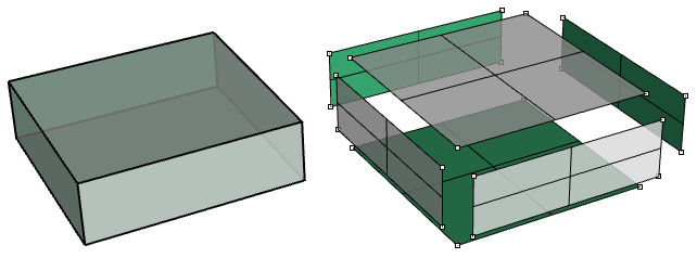
An example polysurface is a simple box that is made out of six untrimmed surfaces joined together.
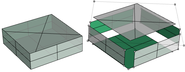
The same box can be made using trimmed surfaces, such as the top one in the following example.
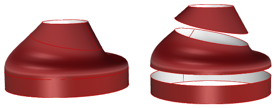
The top and bottom faces of the cylinder in the following example are trimmed from planar surfaces.
We saw that editing NURBS curves and untrimmed surfaces is intuitive and can be done interactively by moving control points. However, editing trimmed surfaces and polysurfaces can be challenging. The main challenge is to be able to maintain joined edges of different faces within the desired tolerance. Neighboring faces that share common edges can be trimmed and do not usually have matching NURBS structure, and therefore modifying the object in a way that deforms that common edge might result in a gap.
Another challenge is that there is typically less control over the outcome, especially when modifying trimmed geometry.
Trimmed surfaces are described in parameter space using the untrimmed underlying surface combined with the 2-D trim curves that evaluate to the 3-D edges within the 3-D surface.
3.10 Tutorials
The following tutorials use the concepts learned in this chapter. They use Rhinoceros 5 and Grasshopper 0.9.
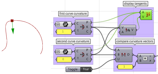
3.10.1 Continuity between curves
Examine the continuity between two input curves. Continuity assumes that the curves meet at the end of the first curve and the start of the second curve.
Input:
Two input curves.
Parameters:
Calculate the following to be able to decide the continuity between two curves:
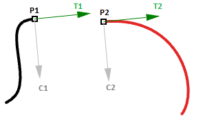
- The end point of the first curve ( $$P1$$)
- The start point of the second curve ( $$P2$$)
- The tangent at the end of the first curve and at the start of the second curve ( $$T1$$ and $$T2$$).
- The curvature at the end of the first curve and at the start of the second curve ( $$C1$$ and $$C2$$).
Solution:
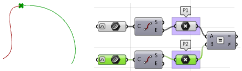
1. Reparameterize the input curves. We do that so that we know that the start of the curve evaluates at
$$t=0$$ and the end at
$$t=1$$.
2. Extract the end and start points of the two curves, and check whether they coincide. If they do, the two curves are at least
$$G0$$ continuous.
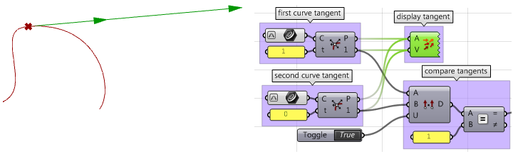
3. Calculate tangents.
4. Compare the tangents using the dot product. Make sure to unitize vectors. If the curves are parallel, then we have at least
$$G1$$ continuity.
5. Calculate curvature vectors.
6. Compare curvature vectors, and if they agree, the two curves are
$$G2$$ continuous.
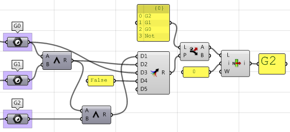
7. Create logic that filters through the three results (G1, G2, and G3) and select the highest continuity.
Using the Grasshopper VBScript component:
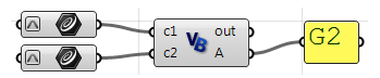
Private Sub RunScript(ByVal c1 As Curve, ByVal c2 As Curve, ByRef A As Object)

  'declare variables
  Dim continuity As New String("")
  Dim t1, t2 As Double
  Dim v_c1, v_c2, c_c1, c_c2 As Vector3d

  'extract start and end points
  Dim end_c1 = c1.PointAtEnd
  Dim start_c2 = c2.PointAtStart

  'check G0 continuity
  If end_c1.DistanceTo(start_c2) = 0 Then
    continuity = "G0"
  End If

  'check G1 continuity
  If continuity = "G0" Then
    'calculate tangents
    v_c1 = c1.TangentAtEnd
    v_c2 = c2.TangentAtStart
    'unitize tangent vectors
    v_c1.Unitize
    v_c2.Unitize
    'compare tangents
    If v_c1 * v_c2 = 1.0 Then
      continuity = "G1"
    End If
  End If

  'check G2 continuity
  If continuity = "G1" Then
    'extract the parameter at start and end of the curves domain
    t1 = c1.Domain.Max
    t2 = c2.Domain.Min
    'calculate curvature
    c_c1 = c1.CurvatureAt(t1)
    c_c2 = c2.CurvatureAt(t2)
    'unitize curvature vectors
    c_c1.Unitize
    c_c2.Unitize
    'compare vectors
    If c_c1 * c_c2 = 1.0 Then
      continuity = "G2"
    End If
  End If

  'Assign output
  A = continuity

End Sub
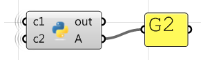
Using the Grasshopper Python component:
#decclare variables
continuity = ""

#extract start and end points
end_c1 = c1.PointAtEnd
start_c2 = c2.PointAtStart

#check G0 continuity
if end_c1.DistanceTo(start_c2) == 0:
    continuity = "G0"

#check G1 continuity
if continuity == "G0":
    #calculate tangents
    v_c1 = c1.TangentAtEnd
    v_c2 = c2.TangentAtStart
    #unitize tangent vectors
    v_c1.Unitize()
    v_c2.Unitize()
    #compare tangents
    dot = v_c1 * v_c2
    if dot == 1.0:
        continuity = "G1"
    else:
        print("Failed G1")
        print(dot)

#check G2 continuity
if continuity == "G1":

    #extract the parameter at start and end of the curves domain
    t1 = c1.Domain.Max
    t2 = c2.Domain.Min
    #calculate curvature
    c_c1 = c1.CurvatureAt(t1)
    c_c2 = c2.CurvatureAt(t2)
    #unitize curvature vectors
    c_c1.Unitize()
    c_c2.Unitize()
    #compare vectors
    dot = c_c1 * c_c2
    if dot == 1.0:
        continuity = "G2"
    else:
        print("Failed G2")
        print(dot)

#assign output
A = continuity
Using the Grasshopper C# component:
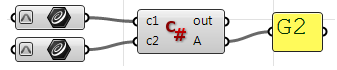
Private Sub RunScript(ByVal c1 As Curve, ByVal c2 As Curve, ByRef A As Object)

    //decalre variables
    string continuity = ("");
    double t1, t2;
    Vector3d v_c1, v_c2, c_c1, c_c2;

    //extract start and end points
    Point3d end_c1 = c1.PointAtEnd;
    Point3d start_c2 = c2.PointAtStart;

    //check G0 continuity
    if( end_c1.DistanceTo(start_c2) == 0){
      continuity = "G0";
    }

    //check G1 continuity
    if( continuity == "G0")
    {
      //calculate tangents
      v_c1 = c1.TangentAtEnd;
      v_c2 = c2.TangentAtStart;
      //unitize tangent vectors
      v_c1.Unitize();
      v_c2.Unitize();
      //compare tangents
      if( v_c1 * v_c2 == 1.0 ){
        continuity = "G1";
      }
    }

    //check G2 continuity
    if( continuity == "G1" )
    {
      //extract the parameter at start and end of the curves domain
      t1 = c1.Domain.Max;
      t2 = c2.Domain.Min;
      //calculate curvature
      c_c1 = c1.CurvatureAt(t1);
      c_c2 = c2.CurvatureAt(t2);
      //unitize curvature vectors
      c_c1.Unitize();
      c_c2.Unitize();
      //compare vectors
      if( c_c1 * c_c2 == 1.0 ){
        continuity = "G2";
      }
    }

    //assign output
    A = continuity;

End Sub
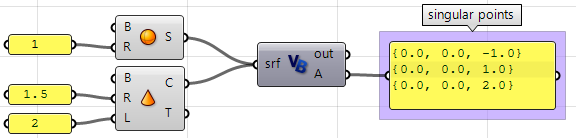
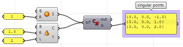
3.10.2 Surfaces with singularity
Extract singular points in a sphere and a cone.
Input:
One sphere and one cone.
Parameters:
Singularity can be detected through analyzing the 2-D parameter space trims that have invalid or zero-length corresponding edges. Those trims ought to be singular.
Solution:
- Traverse through all trims in the input.
- Check if any trim has an invalid edge and flag it as a singular trim.
- Extract point locations in 3-D space.
Using the Grasshopper VB component:
Private Sub RunScript(ByVal srf As Brep, ByRef A As Object)

  'Decalre a new list of points
  Dim singular_points As New List( Of Point3d)

  'Examine all trims in the input
  For Each trim As BrepTrim In srf.Trims

    'Null edge of a trim indicates a singularity
    If trim.Edge Is Nothing Then

      'Find the 2D parameter space point of the start or end of the trim
      Dim pt2d = New Point2d(trim.PointAtStart)

      'Evaluate trim end point on the object surface
      Dim pt3d = trim.Face.PointAt(pt2d.x, pt2d.y)

      'Add 3D point to the list of singular points
      singular_points.Add(pt3d)
    End If

  Next

  'Asign output
  A = singular_points

End Sub
Using the Grasshopper Python component:
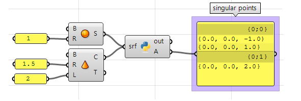
#Decalre a new list of points
singular_points = []

#Examine all trims in the input brep
for trim in srf.Trims:

	#Null edge of a trim indicates a singularity
	if trim.Edge == None:
		#Find the 2D parameter space point at trim start or end
		pt2d = trim.PointAtStart

		#Evaluate trim end point on the object surface
		pt3d = trim.Face.PointAt(pt2d.X, pt2d.Y)

		#Add 3D point to the list of singular points
		singular_points.append(pt3d)

#Asign output
A = singular_points
Using the Grasshopper C# component:
private void RunScript(Brep srf, ref object A)
{
  //Decalre a new list of points
  List < Point3d > singular_points = new List<Point3d>();

  //Examine all trims in the input
  foreach( BrepTrim trim in srf.Trims)
  {
    //Null edge of a trim indicates a singularity
    if( trim.Edge == null)
    {
      //Find the 2D parameter space point of the start or end of the trim
      Point2d pt2d = new Point2d(trim.PointAtStart);

      //Evaluate trim end point on the object surface
      Point3d pt3d = trim.Face.PointAt(pt2d.X, pt2d.Y);

      //Add 3D point to the list of singular points
      singular_points.Add(pt3d);
    }
  }

  //Asign output
  A = singular_points
}
Download Sample Files
Download the download samplesand tutorials archive, containing all the example Grasshopper and code files in this guide.
Next Steps
If you would like to research more, check out the References guide to learn more about the detailed structure of NURBS curves and surfaces.
