
A vector indicates a quantity, such as velocity or force, that has direction and length. Vectors in 3D coordinate systems are represented with an ordered set of three real numbers and look like:
$$\mathbf{\vec v} = <a_1, a_2, a_3>$$1.1 Vector representation
In this document, lower case bold letters with arrow on top will notate vectors. Vector components are also enclosed in angle brackets. Upper case letters will notate points. Point coordinates will always be enclosed by parentheses.
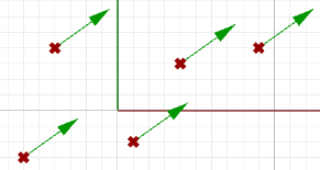
Using a coordinate system and any set of anchor points in that system, we can represent or visualize these vectors using a line-segment representation. An arrowhead shows the vector direction.
For example, if we have a vector that has a direction parallel to the x-axis of a given 3D coordinate system and a length of 5 units, we can write the vector as follows:
$$\mathbf{\vec v} = <5, 0, 0>$$To represent that vector, we need an anchor point in the coordinate system. For example, all of the arrows in the following figure are equal representations of the same vector despite the fact that they are anchored at different locations.
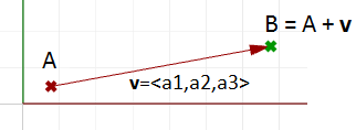
So, how do we define the end points of a line segment that represents a given vector? Let us define an anchor point (A) so that:
$$A = (1, 2, 3)$$And a vector:
$$\mathbf{\vec v} = <5, 6, 7>$$The tip point $$(B)$$ of the vector is calculated by adding the corresponding components from anchor point and vector $$\vec v$$:
$$B = A + \mathbf{\vec v}$$
$$B = (1+5, 2+6, 3+7) $$
$$B = (6, 8, 10)$$
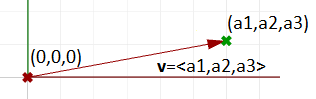
Position vector
One special vector representation uses the $$\text{origin point} (0,0,0)$$ as the vector anchor point. The position vector $$\mathbf{\vec v} = <a_1,a_2,a_3>$$ is represented with a line segment between two points, the origin and the tip point B, so that:
$$\text{Origin point} = (0,0,0)$$
$$B = (a_1,a_2,a_3)$$
Vectors vs. points
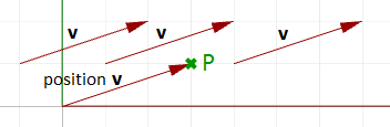
Do not confuse vectors and points. They are very different concepts. Vectors, as we mentioned, represent a quantity that has direction and length, while points indicate a location. For example, the North direction is a vector, while the North Pole is a location (point). If we have a vector and a point that have the same components, such as:
$$\mathbf{\vec v} = <3,1,0>$$
$$P = (3,1,0)$$
We can draw the vector and the point as follows:
Vector length
As mentioned before, vectors have length. We will use $$\vert a \vert$$ to notate the length of a given vector $$ a $$. For example:
$$\mathbf{\vec a} = <4, 3, 0>$$
$$\vert \mathbf{\vec a} \vert = \sqrt{4^2 + 3^2 + 0^2}$$
$$\vert \mathbf{\vec a} \vert = 5$$
In general, the length of a vector $$\mathbf{\vec a} <a_1,a_2,a_3>$$ is calculated as follows:
$$\vert \mathbf{\vec a} \vert = \sqrt{(a_1)^2 + (a_2)^2 + (a_3)^2} $$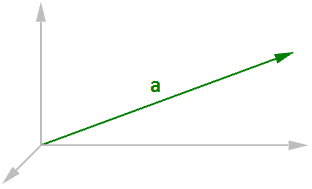
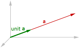
Unit vector
A unit vector is a vector with a length equal to one unit. Unit vectors are commonly used to compare the directions of vectors.
To calculate a unit vector, we need to find the length of the given vector, and then divide the vector components by the length. For example:
$$\mathbf{\vec a} = <4, 3, 0>$$
$$\vert \mathbf{\vec a} \vert = \sqrt{4^2 + 3^2 + 0^2}$$
$$\vert \mathbf{\vec a} \vert = 5 \text{ unit length}$$
If
$$\mathbf{\vec b} = \text{unit vector}$$ of
$$a$$, then:
$$\mathbf{\vec b} = <4/5, 3/5, 0/5>$$
$$\mathbf{\vec b} = <0.8, 0.6, 0>$$
$$\vert \mathbf{\vec b} \vert = \sqrt{0.8^2 + 0.6^2 + 0^2}$$
$$\vert \mathbf{\vec b} \vert = \sqrt{0.64 + 0.36 + 0}$$
$$\vert \mathbf{\vec b} \vert = \sqrt{(1)} = 1 \text{ unit length}$$
In general:
$$\mathbf{\vec a} = <a_1, a_2, a_3>$$The unit vector of $$\mathbf{\vec a} = <a_1/\vert \mathbf{\vec a} \vert , a_2/\vert \mathbf{\vec a} \vert , a_3/\vert \mathbf{\vec a} \vert >$$
1.2 Vector operations
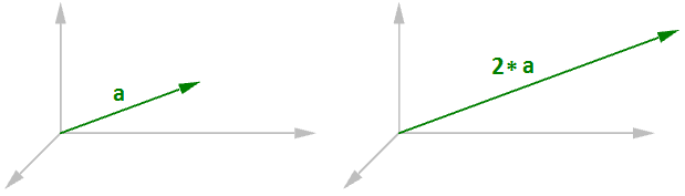
Vector scalar operation
Vector scalar operation involves multiplying a vector by a number. For example:
$$\mathbf{\vec a} = <4, 3, 0>$$
$$2* \mathbf{\vec a} = <24, 23, 2*0>$$
$$2*\mathbf{\vec a} = <8, 6, 0>$$
In general, given vector $$\mathbf{\vec a} = <a_1, a_2, a_3>$$, and a real number $$t$$
$$t*\mathbf{\vec a} = < t* a_1, t* a_2, t* a_3 >$$Vector addition
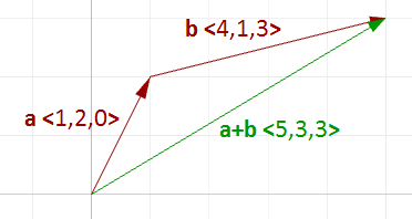
Vector addition takes two vectors and produces a third vector. We add vectors by adding their components.
For example, if we have two vectors:
$$\mathbf{\vec a} = <1, 2, 0> $$
$$\mathbf{\vec b} = <4, 1, 3> $$
$$\mathbf{\vec a}+\mathbf{\vec b} = <1+4, 2+1, 0+3>$$
$$\mathbf{\vec a}+\mathbf{\vec b} = <5, 3, 3>$$
In general, vector addition of the two vectors a and b is calculated as follows:
$$\mathbf{\vec a} = <a_1, a_2, a_3>$$
$$\mathbf{\vec b} = <b_1, b_2, b_3>$$
$$\mathbf{\vec a}+\mathbf{\vec b} = <a_1+b_1, a_2+b_2, a_3+b_3>$$
Vector addition is useful for finding the average direction of two or more vectors. In this case, we usually use same-length vectors. Here is an example that shows the difference between using same-length vectors and different-length vectors on the resulting vector addition:
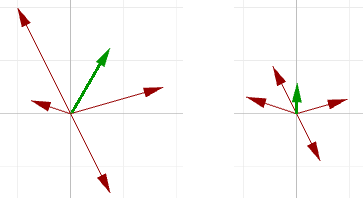
Input vectors are not likely to be same length. In order to find the average direction, you need to use the unit vector of input vectors. As mentioned before, the unit vector is a vector of that has a length equal to 1.
Vector subtraction
Vector subtraction takes two vectors and produces a third vector. We subtract two vectors by subtracting corresponding components. For example, if we have two vectors $$\mathbf{\vec a}$$ and $$\mathbf{\vec b}$$ and we subtract $$\mathbf{\vec b}$$ from $$\mathbf{\vec a}$$, then:
$$\mathbf{\vec a} = <1, 2, 0> $$
$$\mathbf{\vec b} = <4, 1, 4> $$
$$\mathbf{\vec a}-\mathbf{\vec b} = <1-4, 2-1, 0-4>$$
$$\mathbf{\vec a}-\mathbf{\vec b} = <-3, 1, -4> = \mathbf{\mathbf{\vec b}a}$$
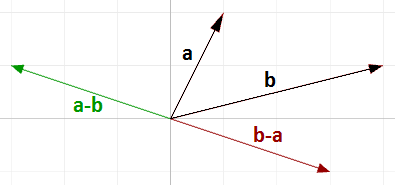
If we subtract $$\mathbf{\vec b}$$ from $$\mathbf{\vec a}$$, we get a different result:
$$\mathbf{\vec b} - \mathbf{\vec a} = <4-1, 1-2, 4-0>$$
$$\mathbf{\vec b} - \mathbf{\vec a} = <3, -1, 4> = \mathbf{\mathbf{\vec a}b}$$
Note that the vector $$\mathbf{\vec b} - \mathbf{\vec a}$$ has the same length as the vector $$\mathbf{\vec a} - \mathbf{\vec b}$$, but goes in the opposite direction.
In general, if we have two vectors, $$\mathbf{\vec a}$$ and $$\mathbf{\vec b}$$, then $$\mathbf{\vec a} - \mathbf{\vec b}$$ is a vector that is calculated as follows:
$$\mathbf{\vec a} = <a_1, a_2, a_3>$$
$$\mathbf{\vec b} = <b_1, b_2, b_3>$$
$$\mathbf{\vec a}-\mathbf{\vec b} = <a_1 - b_1, a_2 - b_2, a_3 - b_3> = \mathbf{\mathbf{\vec b}a}$$
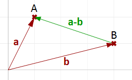
Vector subtraction is commonly used to find vectors between points. So if we need to find a vector that goes from the tip point of the position vector $$\mathbf{\vec b}$$ to the tip point of the position vector $$\mathbf{\vec a}$$, then we use vector subtraction $$(\mathbf{\vec a}-\mathbf{\vec b})$$ as shown in Figure (11).
Vector properties
There are eight properties of vectors. If a, b, and c are vectors, and s and t are numbers, then:
$$\mathbf{\vec a} + \mathbf{\vec b} = \mathbf{\vec b} + \mathbf{\vec a}$$
$$\mathbf{\vec a} + 0 = a$$
$$s * (\mathbf{\vec a} + \mathbf{\vec b}) = s * a + s * \mathbf{\vec b}$$
$$s * t * (\mathbf{\vec a}) = s * (t * \mathbf{\vec a})$$
$$\mathbf{\vec a} + (\mathbf{\vec b} + \mathbf{\vec c}) = (\mathbf{\vec a} + \mathbf{\vec b}) + \mathbf{\vec c}$$
$$\mathbf{\vec a} + (-\mathbf{\vec a}) = 0$$
$$(s + t) * \mathbf{\vec a} = s * \mathbf{\vec a} + t * \mathbf{\vec a}$$
$$1 * \mathbf{\vec a} = \mathbf{\vec a}$$
Vector dot product
The dot product takes two vectors and produces a number. For example, if we have the two vectors a and b so that:
$$\mathbf{\vec a} = <1, 2, 3> $$
$$\mathbf{\vec b} = <5, 6, 7>$$
Then the dot product is the sum of multiplying the components as follows:
$$\mathbf{\vec a} · \mathbf{\vec b} = 1 * 5 + 2 * 6 + 3 * 7$$
$$\mathbf{\vec a} · \mathbf{\vec b} = 38$$
In general, given the two vectors a and b:
$$\mathbf{\vec a} = <a_1, a_2, a_3>$$
$$\mathbf{\vec b} = <b_1, b_2, b_3>$$
$$\mathbf{\vec a} · \mathbf{\vec b} = a_1 * b_1 + a_2 * b_2 + a_3 * b_3$$
We always get a positive number for the dot product between two vectors when they go in the same general direction. A negative dot product between two vectors means that the two vectors go in the opposite general direction.
When calculating the dot product of two unit vectors, the result is always between 1 and +1. For example:
$$\mathbf{\vec a} = <1, 0, 0>$$
$$\mathbf{\vec b} = <0.6, 0.8, 0>$$
$$\mathbf{\vec a} · \mathbf{\vec b} = (1 * 0.6, 0 * 0.8, 0 * 0) = 0.6$$
In addition, the dot product of a vector with itself is equal to that vector’s length to the power of two. For example:
$$\mathbf{\vec a} = <0, 3, 4>$$
$$\mathbf{\vec a} · \mathbf{\vec a} = 0 * 0 + 3 * 3 + 4 * 4 $$
$$\mathbf{\vec a} · \mathbf{\vec a} = 25$$
Calculating the square length of vector $$\mathbf{\vec a}$$ :
$$\vert \mathbf{\vec a} \vert = \sqrt{4^2 + 3^2 + 0^2}$$
$$\vert \mathbf{\vec a} \vert = 5$$
$$\vert \mathbf{\vec a} \vert 2 = 25$$
Vector dot product, lengths, and angles
There is a relationship between the dot product of two vectors and the angle between them.
In general:
$$\mathbf{\vec a} · \mathbf{\vec b} = \vert \mathbf{\vec a} \vert * \vert \mathbf{\vec b} \vert * cos(ө)$$ , or
$$\mathbf{\vec a} · \mathbf{\vec b} / (\vert \mathbf{\vec a} \vert * \vert \mathbf{\vec b} \vert) = cos(ө)$$
Where:
$$ө$$ is the angle included between the vectors.
If vectors a and b are unit vectors, we can simply say:
$$\mathbf{\vec a} · \mathbf{\vec b} = cos(ө)$$And since the cosine of a 90-degree angle is equal to 0, we can say:
For example, if we calculate the dot product of the two orthogonal vectors, World xaxis and yaxis, the result will equal zero.
$$\mathbf{\vec x} = <1, 0, 0>$$
$$\mathbf{\vec y} = <0, 1, 0>$$
$$\mathbf{\vec x} · \mathbf{\vec y} = (1 * 0) + (0 * 1) + (0 * 0)$$
$$\mathbf{\vec x} · \mathbf{\vec y} = 0$$
There is also a relationship between the dot product and the projection length of one vector onto another. For example:
$$\mathbf{\vec a} = <5, 2, 0>$$
$$\mathbf{\vec b} = <9, 0, 0>$$
$$unit(\mathbf{\vec b}) = <1, 0, 0>$$
$$\mathbf{\vec a} · unit(\mathbf{\vec b}) = (5 * 1) + (2 * 0) + (0 * 0) $$
$$\mathbf{\vec a} · unit(\mathbf{\vec b}) = 2 (\text{which is equal to the projection length of mathbf{\vec a} onto mathbf{\vec b}})$$
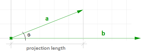
In general, given a vector a and a non-zero vector b, we can calculate the projection length pL of vector a onto vector b using the dot product.
$$pL = \vert \mathbf{\vec a} \vert * cos(ө) $$
$$pL = \mathbf{\vec a} · unit(\mathbf{\vec b})$$
Dot product properties
If $$\mathbf{\vec a}$$, $$\mathbf{\vec b}$$, and $$\mathbf{\vec c}$$ are vectors and s is a number, then:
$$\mathbf{\vec a} · \mathbf{\vec a} = \vert \mathbf{\vec a} \vert ^2$$
$$\mathbf{\vec a} · (\mathbf{\vec b} + \mathbf{\vec c}) = \mathbf{\vec a} · \mathbf{\vec b} + \mathbf{\vec a} · \mathbf{\vec c}$$
$$0 · \mathbf{\vec a} = 0$$
$$\mathbf{\vec a} · \mathbf{\vec b} = \mathbf{\vec b} · \mathbf{\vec a}$$
$$(s * \mathbf{\vec a}) · \mathbf{\vec b} = s * (\mathbf{\vec a} · \mathbf{\vec b}) = \mathbf{\vec a} · (s * \mathbf{\vec b})$$
Vector cross product
The cross product takes two vectors and produces a third vector that is orthogonal to both.
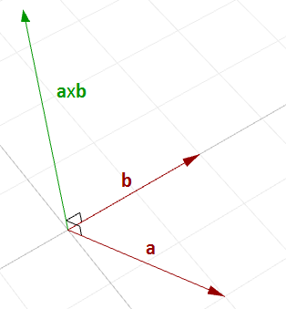
For example, if you have two vectors lying on the World xy-plane, then their cross product is a vector perpendicular to the xy-plane going either in the positive or negative World z-axis direction. For example:
$$\mathbf{\vec a} = <3, 1, 0>$$
$$\mathbf{\vec b} = <1, 2, 0>$$
$$\mathbf{\vec a} × \mathbf{\vec b} = < (1 * 0 – 0 * 2), (0 * 1 - 3 * 0), (3 * 2 - 1 * 1) > $$
$$\mathbf{\vec a} × \mathbf{\vec b} = <0, 0, 5>$$
You will probably never need to calculate a cross product of two vectors by hand, but if you are curious about how it is done, continue reading; otherwise you can safely skip this section. The cross product $$a × b$$ is defined using determinants. Here is a simple illustration of how to calculate a determinant using the standard basis vectors:
$$ \color {red}{i} = <1, 0, 0>$$
$$ \color {blue}{j} = <0,1, 0>$$
$$ \color {green}{k} = <0, 0, 1>$$
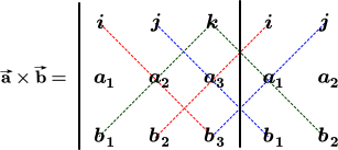
The cross product of the two vectors $$\mathbf{\vec a} = <a1, a2, a3>$$ and $$\mathbf{\vec b} = <b1, b2, b3>$$ is calculated as follows using the above diagram:
$$\mathbf{\vec a} × \mathbf{\vec b} = \color {red}{i (a_2 * b_3)} + \color {blue}{ j (a_3 * b_1)} + \color {green}{k(a_1 * b_2)} - \color {green}{k (a_2 * b_1)} - \color {red}{i (a_3 * b_2)} -\color {blue}{ j (a_1 * b_3)}$$
$$\mathbf{\vec a} × \mathbf{\vec b} = \color {red}{i (a_2 * b_3 - a_3 * b_2)} + \color {blue}{j (a_3 * b_1 - a_1 * b_3)} +\color {green}{k (a_1 * b_2 - a_2 * b_1)}$$
$$\mathbf{\vec a} × \mathbf{\vec b} = <\color {red}{a_2 * b_3 – a_3 * b_2}, \color {blue}{a_3 * b_1 - a_1 * b_3}, \color {green}{a_1 * b_2 - a_2 * b_1} >$$
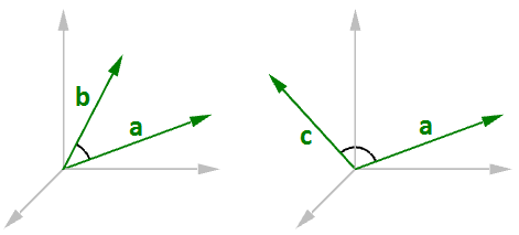
Cross product and angle between vectors
There is a relationship between the angle between two vectors and the length of their cross product vector. The smaller the angle (smaller sine); the shorter the cross product vector will be. The order of operands is important in vectors cross product. For example:
$$\mathbf{\vec a} = <1, 0, 0>$$
$$\mathbf{\vec b} = <0, 1, 0>$$
$$\mathbf{\vec a} × \mathbf{\vec b} = <0, 0, 1>$$
$$\mathbf{\vec b} × \mathbf{\vec a} = <0, 0, -1>$$
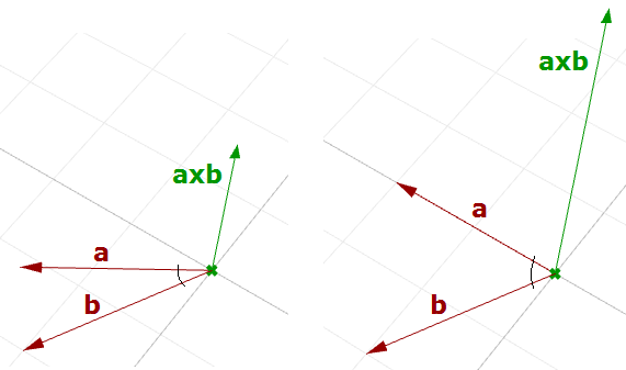
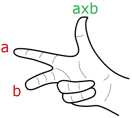
In Rhino’s right-handed system, the direction of $$\mathbf{\vec a} × \mathbf{\vec b}$$ is given by the right-hand rule (where $$\mathbf{\vec a}$$ = index finger, $$\mathbf{\vec b}$$ = middle finger, and $$\mathbf{\vec a} × \mathbf{\vec b}$$ = thumb).
In general, for any pair of 3-D vectors $$\mathbf{\vec a}$$ and $$\mathbf{\vec b}$$:
$$\vert \mathbf{\vec a} × \mathbf{\vec b} \vert = \vert \mathbf{\vec a} \vert \vert \mathbf{\vec b} \vert sin(ө)$$Where:
$$ө$$ is the angle included between the position vectors of $$\mathbf{\vec a}$$ and $$\mathbf{\vec b}$$
If a and b are unit vectors, then we can simply say that the length of their cross product equals the sine of the angle between them. In other words:
$$\vert \mathbf{\vec a} × \mathbf{\vec b} \vert = sin(ө)$$The cross product between two vectors helps us determine if two vectors are parallel. This is because the result is always a zero vector.
Cross product properties
If
$$\mathbf{\vec a}$$,
$$\mathbf{\vec b}$$, and
$$\mathbf{\vec c}$$ are vectors, and
$$s$$ is a number, then:
$$\mathbf{\vec a} × \mathbf{\vec b} = -\mathbf{\vec b} × \mathbf{\vec a}$$
$$(s * \mathbf{\vec a}) × \mathbf{\vec b} = s * (\mathbf{\vec a} × \mathbf{\vec b}) = \mathbf{\vec a} × (s * \mathbf{\vec b})$$
$$\mathbf{\vec a} × (\mathbf{\vec b} + \mathbf{\vec c}) = \mathbf{\vec a} × \mathbf{\vec b} + \mathbf{\vec a} × \mathbf{\vec c}$$
$$(\mathbf{\vec a} + \mathbf{\vec b}) × \mathbf{\vec c} = \mathbf{\vec a} × \mathbf{\vec c} + \mathbf{\vec b} × \mathbf{\vec c}$$
$$\mathbf{\vec a} · (\mathbf{\vec b} × \mathbf{\vec c}) = (\mathbf{\vec a} × \mathbf{\vec b}) · \mathbf{\vec c}$$
$$\mathbf{\vec a} × (\mathbf{\vec b} × \mathbf{\vec c}) = (\mathbf{\vec a} · \mathbf{\vec c}) * \mathbf{\vec b} – (\mathbf{\vec a} · \mathbf{\vec b}) * \mathbf{\vec c}$$
1.3 Vector equation of line
The vector line equation is used in 3D modeling applications and computer graphics.
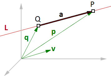
For example, if we know the direction of a line and a point on that line, then we can find any other point on the line using vectors, as in the following:
$$\overline{L} = line$$
$$\mathbf{\vec v} = <a, b, c>$$ line direction unit vector
$$Q = (x_0, y_0, z_0)$$ line position point
$$P = (x, y, z)$$ any point on the line
We know that:
$$\mathbf{\vec a} = t *\mathbf{\vec v}$$ (2)
$$\mathbf{\vec p} = \mathbf{\vec q} + \mathbf{\vec a}$$ (1)
From 1 and 2:
$$\mathbf{\vec p} = \mathbf{\vec q} + t * \mathbf{\vec v}$$ (3)
However, we can write (3) as follows:
$$<x, y, z> = <x_0, y_0, z_0> + <t * a, t * b, t * c>$$
$$<x, y, z> = <x_0 + t * a, y_0 + t * b, z_0 + t * c>$$
Therefore:
$$x = x_0 + t * a$$
$$y = y_0 + t * b$$
$$z = z_0 + t * c$$
Which is the same as:
$$P = Q + t * \mathbf{\vec v}$$Another common example is to find the midpoint between two points. The following shows how to find the midpoint using the vector equation of a line:
$$\mathbf{\vec q}$$ is the position vector for point
$$Q$$
$$\mathbf{\vec p}$$ is the position vector for point
$$P$$
$$\mathbf{\vec a}$$ is the vector going from
$$Q \rightarrow P$$
From vector subtraction, we know that:
$$\mathbf{\vec a} = \mathbf{\vec p} - \mathbf{\vec q}$$From the line equation, we know that:
$$M = Q + t * \mathbf{\vec a}$$And since we need to find midpoint, then:
$$t = 0.5$$Hence we can say:
$$M = Q + 0.5 * \mathbf{\vec a}$$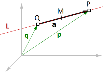
In general, you can find any point between $$Q$$ and $$P$$ by changing the $$t$$ value between 0 and 1 using the general equation:
$$M = Q + t * (P - Q)$$1.4 Vector equation of a plane
One way to define a plane is when you have a point and a vector that is perpendicular to the plane. That vector is usually referred to as normal to the plane. The normal points in the direction above the plane.
One example of how to calculate a plane normal is when we know three non-linear points on the plane.
In Figure (16), given:
$$A$$ = the first point on the plane
$$B$$ = the second point on the plane
$$C$$ = the third point on the plane
And:
$$\mathbf{\vec a} $$ = a position vector of point
$$A$$
$$\mathbf{\vec b}$$ = a position vector of point
$$B$$
$$\mathbf{\vec c}$$ = a position vector of point
$$C$$
We can find the normal vector $$\mathbf{\vec n}$$ as follows:
$$\mathbf{\vec n} = (\mathbf{\vec b} - \mathbf{\vec a}) × (\mathbf{\vec c} - \mathbf{\vec a})$$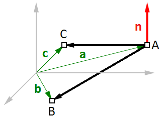
We can also derive the scalar equation of the plane using the vector dot product:
$$\mathbf{\vec n} · (\mathbf{\vec b} - \mathbf{\vec a}) = 0$$If:
$$\mathbf{\vec n} = <a, b, c>$$
$$\mathbf{\vec b} = <x, y, z>$$
$$ \mathbf{\vec a} = <x_0, y_0, z_0>$$
Then we can expand the above:
$$<a, b, c> · <x-x_0, y-y_0, z-z_0 > = 0$$Solving the dot product gives the general scalar equation of a plane:
$$a * (x - x_0) + b * (y - y_0) + c * (z - z_0) = 0$$1.5 Tutorials
All the concepts we reviewed in this chapter have a direct application to solving common geometry problems encountered when modeling. The following are stepbystep tutorials that use the concepts learned in this chapter using Rhinoceros and Grasshopper (GH).
1.5.1 Face direction
Given a point and a surface, how can we determine whether the point is facing the front or back side of that surface?
Input:
- a surface
- a point
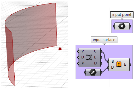
Parameters:
The face direction is defined by the surface normal direction. We will need the following information:
- The surface normal direction at a surface location closest to the input point.
- A vector direction from the closest point to the input point.
Compare the above two directions, if going the same direction, the point is facing the front side, otherwise it is facing the back.
Solution:
1. Find the closest point location on the surface relative to the input point using the Pull component. This will give us the uv location of the closest point, which we can then use to evaluate the surface and find its normal direction.
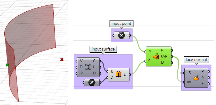
2. We can now use the closest point to draw a vector going towards the input point. We can also draw:
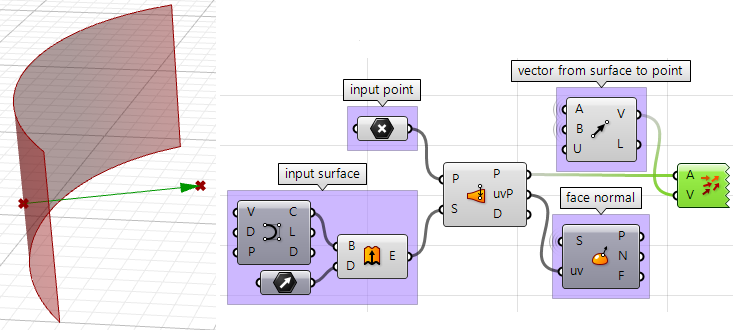
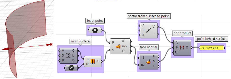
3. We can compare the two vectors using the dot product. If the result is positive, the point is in front of the surface. If the result is negative, the point is behind the surface.
The above steps can also be solved using other scripting languages. Using the Grasshopper VB component:
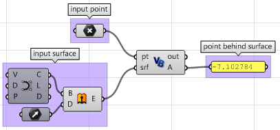
Private Sub RunScript(ByVal pt As Point3d, ByVal srf As Surface, ByRef A As Object)

  'Declare variables
  Dim u, v As Double
  Dim closest_pt As Point3d

  'get closest point u, v
  srf.ClosestPoint(pt, u, v)

  'get closest point
  closest_pt = srf.PointAt(u, v)

  'calculate direction from closest point to test point
  Dim dir As New Vector3d(pt - closest_pt)

  'calculate surface normal
  Dim normal = srf.NormalAt(u, v)

  'compare the two directions using the dot product
  A = dir * normal
End Sub
Using the Grasshopper Python component with RhinoScriptSyntax:
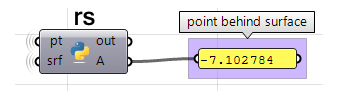
import rhinoscriptsyntax as rs #import RhinoScript library

#find the closest point
u, v = rs.SurfaceClosestPoint(srf, pt)

#get closest point
closest_pt = rs.EvaluateSurface(srf, u, v)

#calculate direction from closest point to test point
dir = rs.PointCoordinates(pt) - closest_pt

#calculate surface normal
normal = rs.SurfaceNormal(srf, [u, v])

#compare the two directions using the dot product
A = dir * normal
Using the Grasshopper Python component with RhinoCommon only:
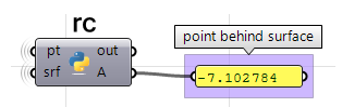
#find the closest point
found, u, v = srf.ClosestPoint(pt)

if found:

    #get closest point
    closest_pt = srf.PointAt(u, v)

    #calculate direction from closest point to test point
    dir = pt - closest_pt

    #calculate surface normal
    normal = srf.NormalAt(u, v)

    #compare the two directions using the dot product
    A = dir * normal
Using the Grasshopper C# component:
private void RunScript(Point3d pt, Surface srf, ref object A)
{
  //Declare variables
  double u, v;
  Point3d closest_pt;

  //get closest point u, v
  srf.ClosestPoint(pt, out u, out v);

  //get closest point
  closest_pt = srf.PointAt(u, v);

  //calculate direction from closest point to test point
  Vector3d dir = pt - closest_pt;

  //calculate surface normal
  Vector3d normal = srf.NormalAt(u, v);

  //compare the two directions using the dot product
  A = dir * normal;
}
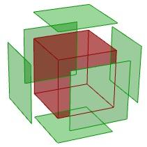
1.5.2 Exploded box
The following tutorial shows how to explode a polysurface. This is what the final exploded box looks like:
Input:
Identify the input, which is a box. We will use the Box parameter in GH:
Parameters:
- Think of all the parameters we need to know in order to solve this tutorial.
- The center of explosion.
- The box faces we are exploding.
- The direction in which each face is moving.
Once we have identified the parameters, it is a matter of putting it together in a solution by piecing together the logical steps to reach an answer.
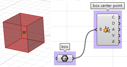
Solution:
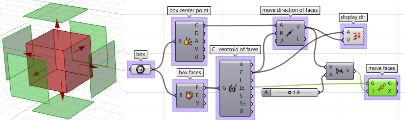
1. Find the center of the box using the Box Properties component in GH:
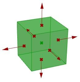
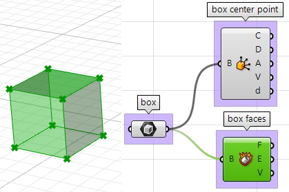
2. Extract the box faces with the Deconstruct Brep component:
3. The direction we move the faces is the tricky part. We need to first find the center of each face, and then define the direction from the center of the box towards the center of each face as follows:
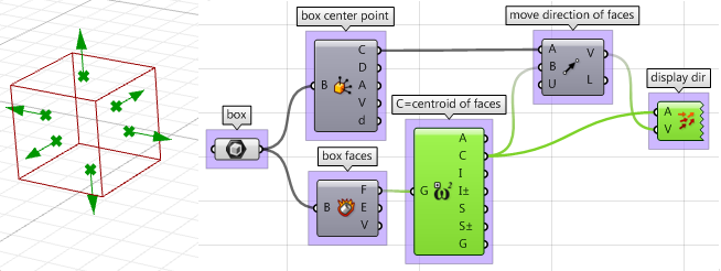
4. Once we have all the parameters scripted, we can use the Move component to move the faces in the appropriate direction. Just make sure to set the vectors to the desired amplitude, and you will be good to go.
The above steps can also be solved using VB script, C# or Python. Following is the solution using these scripting languages.
Using the Grasshopper VB component:
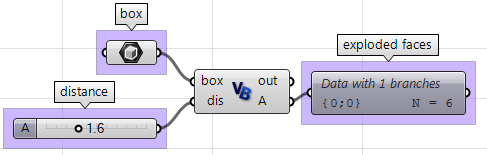
Private Sub RunScript(ByVal box As Brep, ByVal dis As Double, ByRef A As Object)

    'get the brep center
    Dim area As Rhino.Geometry.AreaMassProperties
    area = Rhino.Geometry.AreaMassProperties.Compute(box)

    Dim box_center As Point3d
    box_center = area.Centroid

    'get a list of faces
    Dim faces As Rhino.Geometry.Collections.BrepFaceList = box.Faces

    'decalre variables
    Dim center As Point3d
    Dim dir As Vector3d
    Dim exploded_faces As New List( Of Rhino.Geometry.Brep )
    Dim i As Int32
    'loop through all faces

    For i = 0 To faces.Count() - 1
      'extract each of the face
      Dim extracted_face As Rhino.Geometry.Brep = box.Faces.ExtractFace(i)

      'get the center of each face
      area = Rhino.Geometry.AreaMassProperties.Compute(extracted_face)
      center = area.Centroid

      'calculate move direction (from box centroid to face center)
      dir = center - box_center
      dir.Unitize()
      dir *= dis

      'move the extracted face
      extracted_face.Transform(Transform.Translation(dir))

      'add to exploded_faces list
      exploded_faces.Add(extracted_face)
    Next

    'assign exploded list of faces to output
    A = exploded_faces
  End Sub
Using the Grasshopper Python component with RhinoCommon:
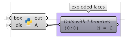
import Rhino

#get the brep center
area = Rhino.Geometry.AreaMassProperties.Compute(box)
box_center = area.Centroid

#get a list of faces
faces = box.Faces

#decalre variables
exploded_faces = []

#loop through all faces
for i, face in enumerate(faces):

	#get a duplicate of the face
	extracted_face = faces.ExtractFace(i)

	#get the center of each face
	area = Rhino.Geometry.AreaMassProperties.Compute(extracted_face)
	center = area.Centroid

	#calculate move direction (from box centroid to face center)
	dir = center - box_center
	dir.Unitize()
	dir *= dis

	#move the extracted face
	move = Rhino.Geometry.Transform.Translation(dir)
	extracted_face.Transform(move)

	#add to exploded_faces list
	exploded_faces.append(extracted_face)

#assign exploded list of faces to output
A = exploded_faces
Using the Grasshopper C# component:
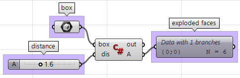
private void RunScript(Brep box, double dis, ref object A)
{

    //get the brep center
  Rhino.Geometry.AreaMassProperties area =        Rhino.Geometry.AreaMassProperties.Compute(box);
  Point3d box_center = area.Centroid;

  //get a list of faces
  Rhino.Geometry.Collections.BrepFaceList faces = box.Faces;

  //decalre variables
  Point3d center;   Vector3d dir;
  List<Rhino.Geometry.Brep> exploded_faces = new List<Rhino.Geometry.Brep>();

  //loop through all faces   for( int i = 0; i < faces.Count(); i++ )
  {
    //extract each of the face
    Rhino.Geometry.Brep extracted_face = box.Faces.ExtractFace(i);

    //get the center of each face
    area = Rhino.Geometry.AreaMassProperties.Compute(extracted_face);
    center = area.Centroid;

    //calculate move direction (from box centroid to face center)
    dir = center - box_center;
    dir.Unitize();
    dir *= dis;

    //move the extracted face
    extracted_face.Transform(Transform.Translation(dir));

    //add to exploded_faces list
    exploded_faces.Add(extracted_face);
  }

  //assign exploded list of faces to output
  A = exploded_faces;
}
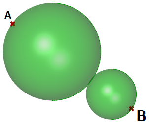
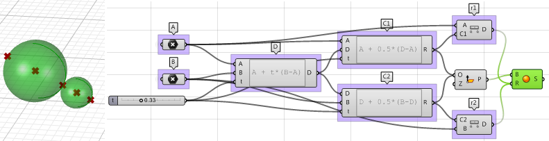
1.5.3 Tangent spheres
This tutorial will show how to create two tangent spheres between two input points. This is what the result looks like:
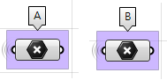
Input:
Two points (
$$A$$ and
$$B$$) in the 3-D coordinate system.
Parameters: The following is a diagram of the parameters that we will need in order to solve the problem: $$A$$ tangent point $$D$$ between the two spheres, at some $$t$$ parameter (0-1) between points $$A$$ and $$B$$.
- The center of the first sphere or the midpoint $$C1$$ between $$A$$ and $$D$$.
- The center of the second sphere or the midpoint $$C2$$ between $$D$$ and $$B$$.
- The radius of the first sphere $$(r1)$$ or the distance between $$A$$ and $$C1$$.
- The radius of the second sphere $$(r2)$$ or the distance between $$D$$ and $$C2$$.
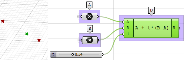
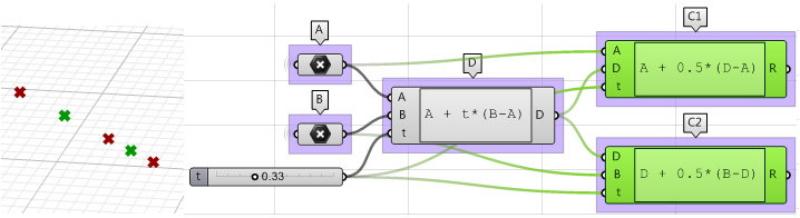
Solution:
1. Use the Expression component to define point $$D$$ between $$A$$ and $$B$$ atsome parameter $$t$$. The expression we will use is based onthe vector equation of a line:
$$D = A + t*(B-A)$$$$B-A$$ : is the vector that goes from point $$A$$ to point $$B$$ using the vector subtraction operation.
$$t*(B-A)$$ : where $$t$$ is between 0 and 1 to get us a location on the vector.
$$A+t*(B-A)$$ : gets apoint on the vector between A and B.
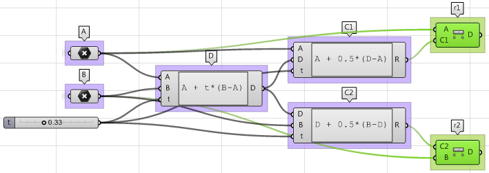
2. Use the Expression component to also define the mid points $$C1$$ and $$C2$$ .
3. The first sphere radius $$(r1)$$ and the second sphere radius $$(r2)$$ can be calculated using the Distance component.
4. The final step involves creating the sphere from a base plane and radius. We need to make sure the origins are hooked to $$C1$$ and $$C2$$ and the radius from $$r1$$ and $$r2$$.
Using the Grasshopper VB component:
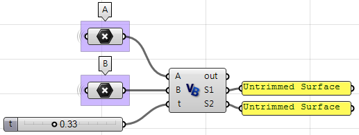
Private Sub RunScript(ByVal A As Point3d, ByVal B As Point3d, ByVal t As Double, ByRef S1 As Object, ByRef S2 As Object)

  'declare variables
  Dim D, C1, C2 As Rhino.Geometry.Point3d
  Dim r1, r2 As Double

  'find a point between A and B
  D = A + t * (B - A)

  'find mid point between A and D
  C1 = A + 0.5 * (D - A)

  'find mid point between D and B
  C2 = D + 0.5 * (B - D)
  'find spheres radius
  r1 = A.DistanceTo(C1)
  r2 = B.DistanceTo(C2)

  'create spheres and assign to output
  S1 = New Rhino.Geometry.Sphere(C1, r1)
  S2 = New Rhino.Geometry.Sphere(C2, r2)

End Sub
Using Python component:
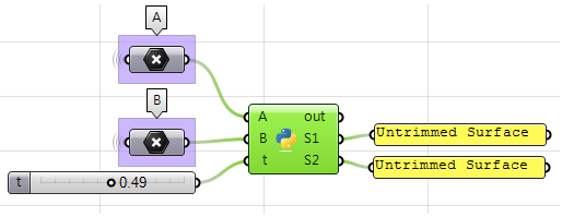
import Rhino

#find a point between A and B
D = A + t * (B - A)

#find mid point between A and D
C1 = A + 0.5 * (D - A)

#find mid point between D and B
C2 = D + 0.5 * (B - D)

#find spheres radius
r1 = A.DistanceTo(C1)
r2 = B.DistanceTo(C2)

#create spheres and assign to output
S1 = Rhino.Geometry.Sphere(C1, r1)
S2 = Rhino.Geometry.Sphere(C2, r2)
Using the Grasshopper C# component:
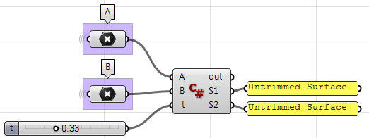
private void RunScript(Point3d A, Point3d B, double t, ref object S1, ref object S2)
{
  //declare variables
  Rhino.Geometry.Point3d D, C1, C2;
  double r1, r2;

  //find a point between A and B
  D = A + t * (B - A);

  //find mid point between A and D
  C1 = A + 0.5 * (D - A);

  //find mid point between D and B
  C2 = D + 0.5 * (B - D);

  //find spheres radius
  r1 = A.DistanceTo(C1);
  r2 = B.DistanceTo(C2);

  //create spheres and assign to output
  S1 = new Rhino.Geometry.Sphere(C1, r1);
  S2 = new Rhino.Geometry.Sphere(C2, r2);
}
Download Sample Files
Download the download samplesand tutorials archive, containing all the example Grasshopper and code files in this guide.
Next Steps
Now that you know vector math, check out the Matrices and Transformations guide to learn more about the moving, rotating and scaling objects..
