by Rajaa Issa (Last updated:  Monday, July 15, 2024)

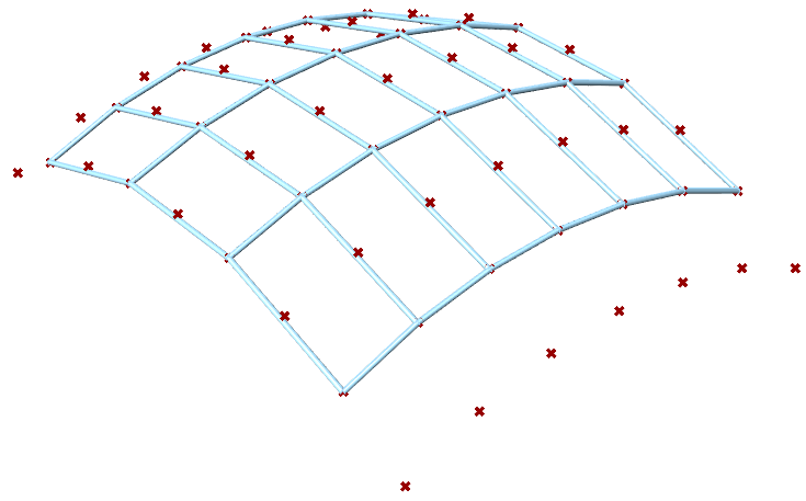
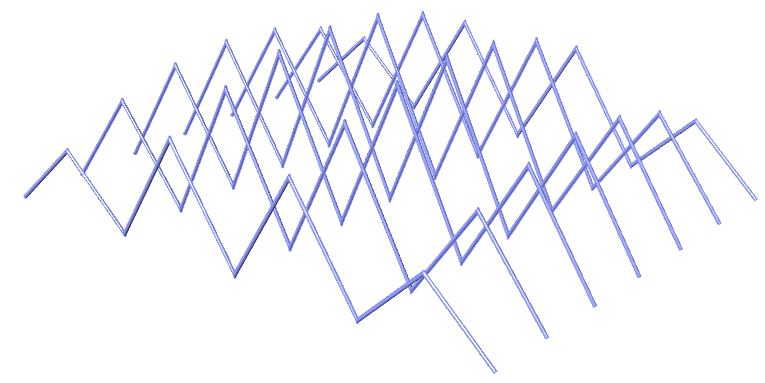
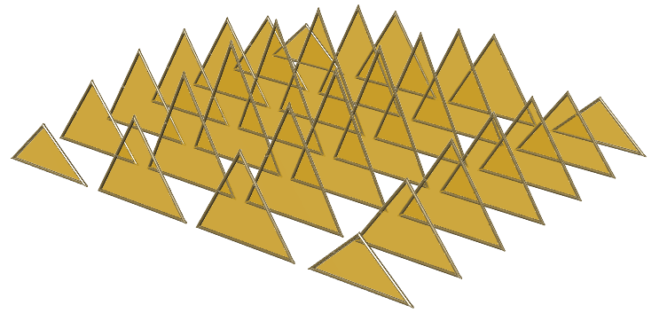
This chapter is devoted to the advanced data structure in GH, namely the data trees, and different ways to generate and manage them. The aim is to start to appreciate when and how to use tree structures, and best practices to effectively use and manipulate them.

3.1 The Grasshopper data structure

3.1.1 Introduction

Introduction to data trees

In programming, there are many data structures to govern how data is stored and accessed. The most common data structures are variables, arrays, and nested arrays. There are other data structures that are optimised for specific purposes such as data sorting or mining. In Grasshopper, there is only one structure to store data, and that is the data tree. Hold on, what about what we have learned so far: single item and list of items? Well, in GH, those are nothing but simple trees. A single item is a tree with one branch, that has one element, and a list is a tree with one branch that has a number of elements. It is actually pretty elegant to be able to fit all data in one unifying data structure, but at the same time, this requires the user to be aware and vigilant about how their data structure changes between operations, and how that can affect intended results. This chapter attempts to demystify the data tree of Grasshopper.

3.1.2 Processing data trees

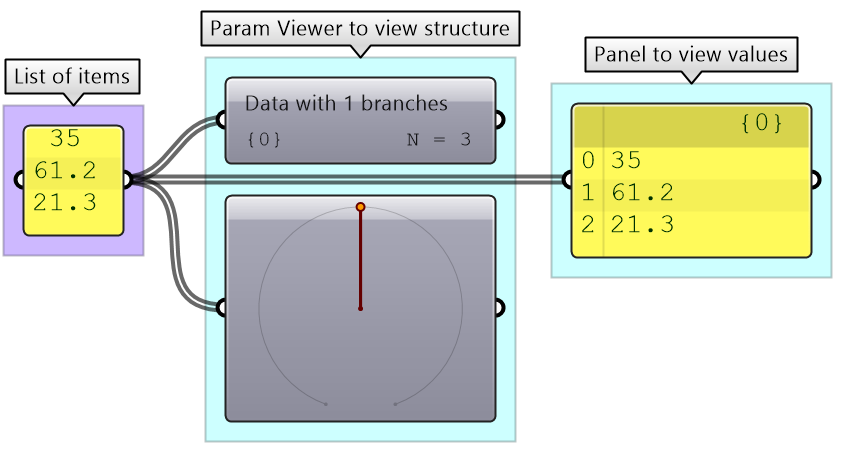
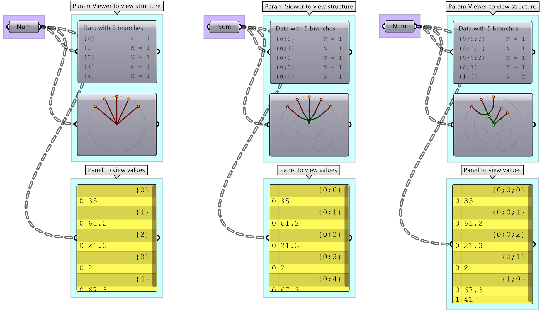
We used the Panel and Parameter Viewer components to view the data structure. We will use both extensively to show how data is stored. Let’s start with a single item input. The Parameter Viewer has two display modes, one with text and one that is graphical. You can see that the single item input is stored in one branch that has only one item.

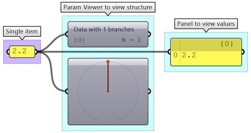
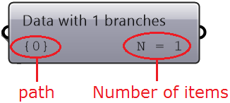
The Parameter Viewer shows each branch address (called “Path”), and the number of elements in that branch as shown in Figure (52).

A list of items is typically stored in a tree with one branch. Figure (53). However, the three items can also be stored in three different branches. Figure (54).

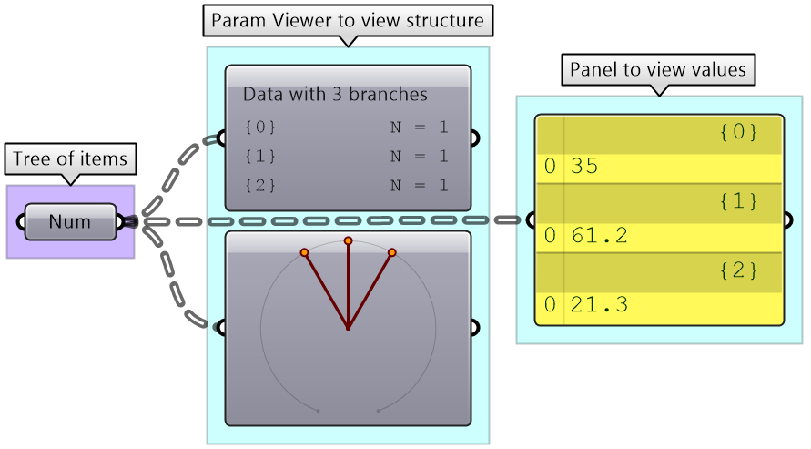
The key to understanding the Grasshopper data structure is to be able to answer the following question:
What is the significance of storing x number of values in one branch vs using x number of branches to store one value in each branch?
The data structure informs GH components about how to match input values. In other words, components may process data differently based on their structure. The following example illustrates how different data structures for the same set of values can affect the result.

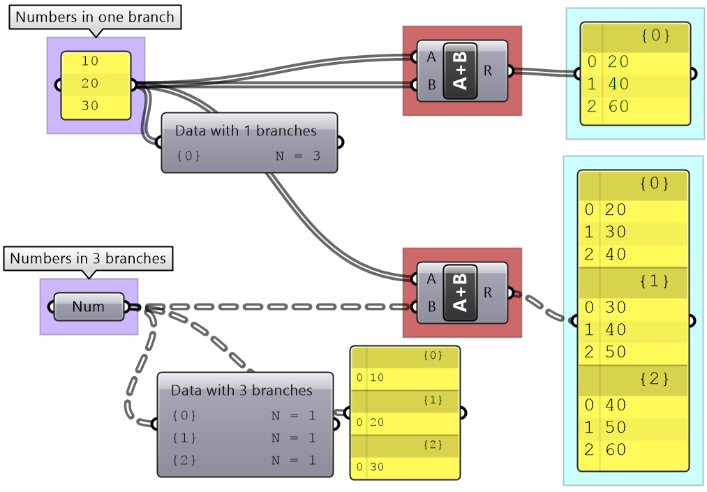
We will elaborate on data tree matching later, but you can already see that GH components do pay attention to the data structure and the result can vary considerably based on it. This is one of the complications inherited in using one unifying data structure in a programming language.

3.1.3 Data tree notation

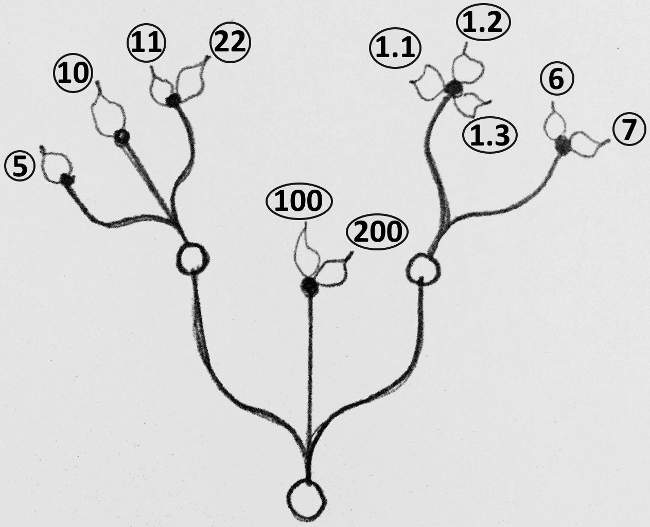
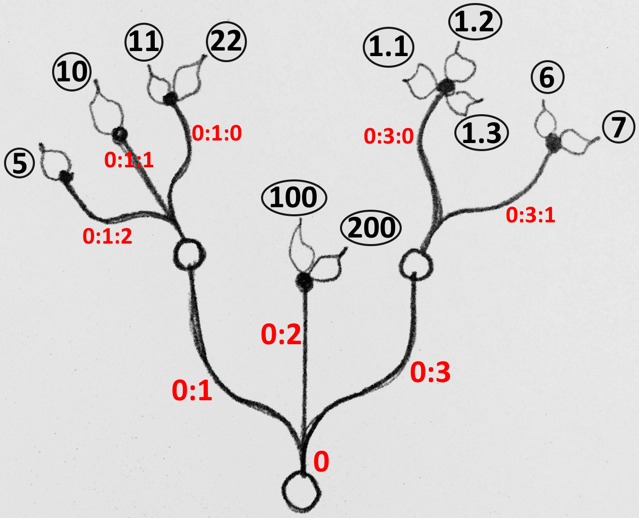
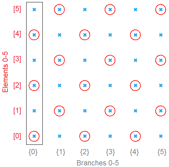
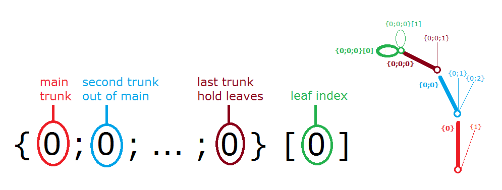
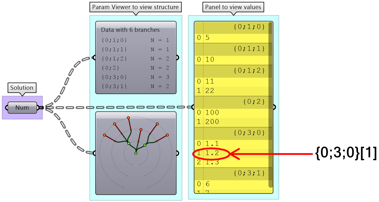
The first step to understanding data trees is to learn the GH notation of trees. As we have seen from the examples, trees consist of branches, and each branch holds a number of elements. The address or path of each branch is represented with integers separated by semicolons and enclosed in curly brackets. The index of each element is enclosed by square brackets. This diagram shows a breakdown of the address of elements in trees.

Here are a few examples of various tree structures and how they show in the Parameter Viewer and the Panel.

Tutorial 3.1.1 Data tree
1. In the tree, what is the full address to the item 1.2? Note that order of branches and leaves is always from left to right going clockwise 2. Construct the tree of numbers shown in the image below using the Number parameter only.
Solution... The path to 1.2 is: { 0 ; 3 ; 0} [ 1 ] Note: The three branches from the main trunk are set here to 0:1, 0:2, and 0:3. They also could have been 0:0, 0:1 and 0:2. Both are correct.

3.2 Generating trees

Generate data trees

There are many ways to generate complex data trees. Some explicit, but mostly as a result of some processes, and this is why you need to always be aware of the data structures of output before using it as input downstream. It is possible to enter the data and set the data structure directly inside any Grasshopper parameter. Once set, it is relatively hard to change and therefore is best suited for a constant input. The following is an example of how to set a data tree directly inside a parameter.

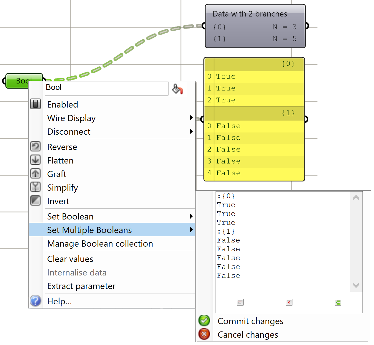
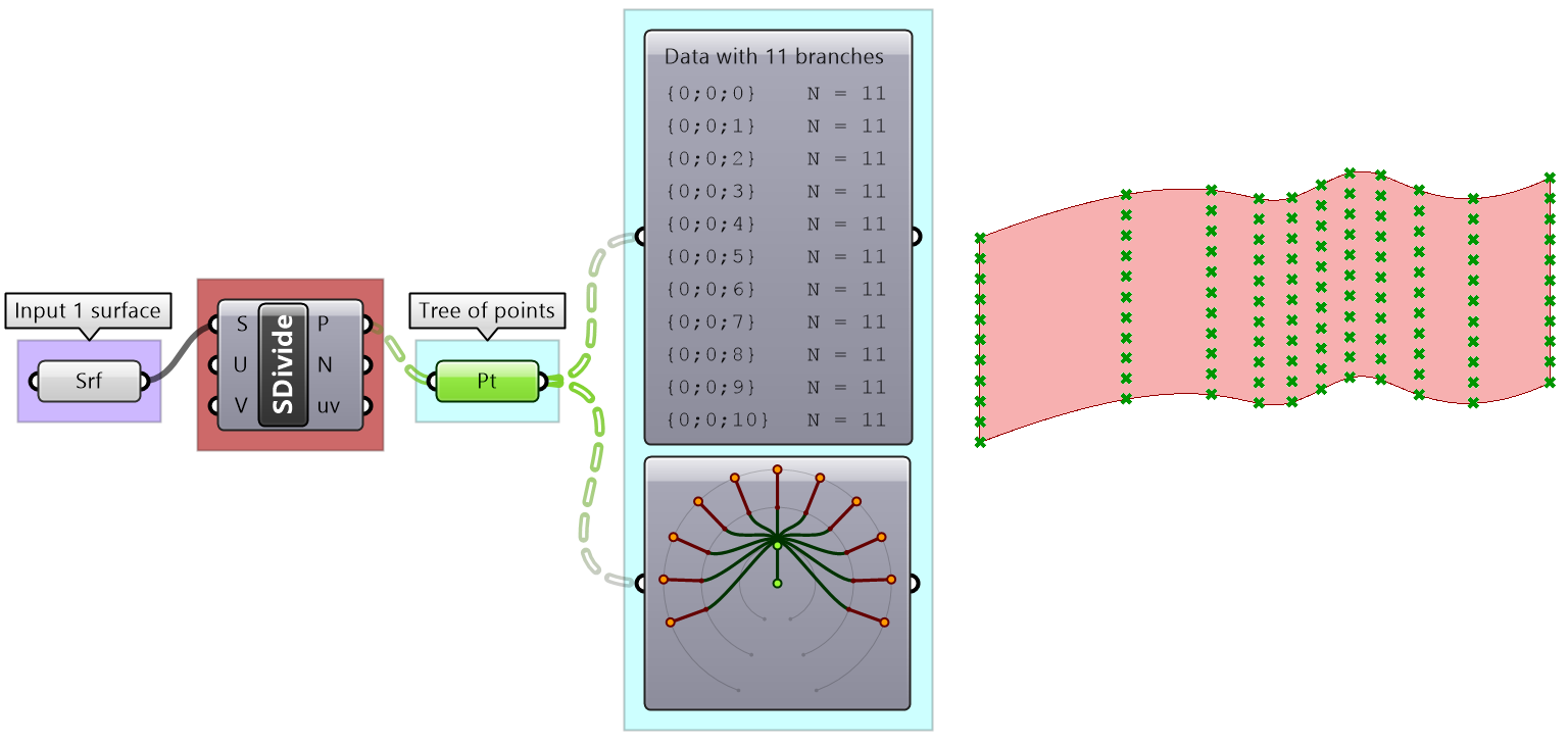
There are many components that generate data trees such as Grid and DivideSrf, and others that combine lists into a tree structure such as Entwine. Also all the components that produce lists can also create a tree if the input is a list. For example, if you input more than one curve into the DivideCrv component, we get a tree of points.

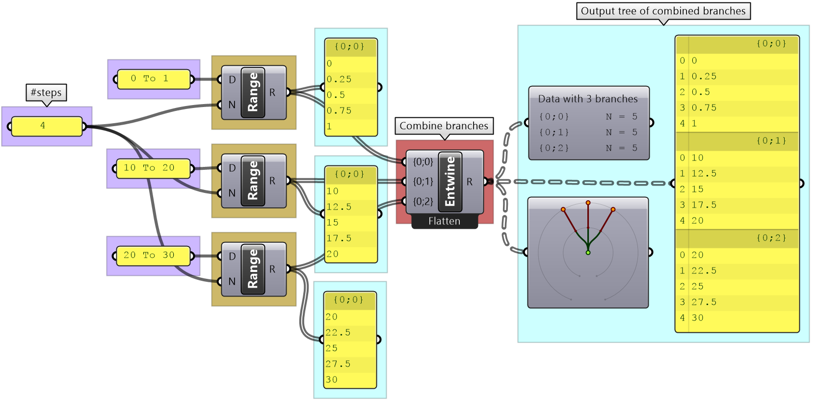
All components that generate lists of numbers (such as Range and Series) can also generate trees when given a list of input.

Perhaps one of the most common cases to generate a tree is when dividing a list of curves to generate a grid of points. So the input is one list and the output is a tree.

Tutorial 3-2-1: Generating trees
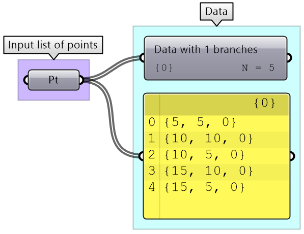
Given the following list of points, construct a number tree with 3 branches, one for each coordinate.
Solution... Each input point is a single data item that contains 3 numbers (coordinates). We know we would like to isolate each coordinate into a separate list, then combine them into one data structure. Hence we need to first deconstruct input points (use Deconstruct of pDecon component), then combine the lists into one structure (use Entwine component).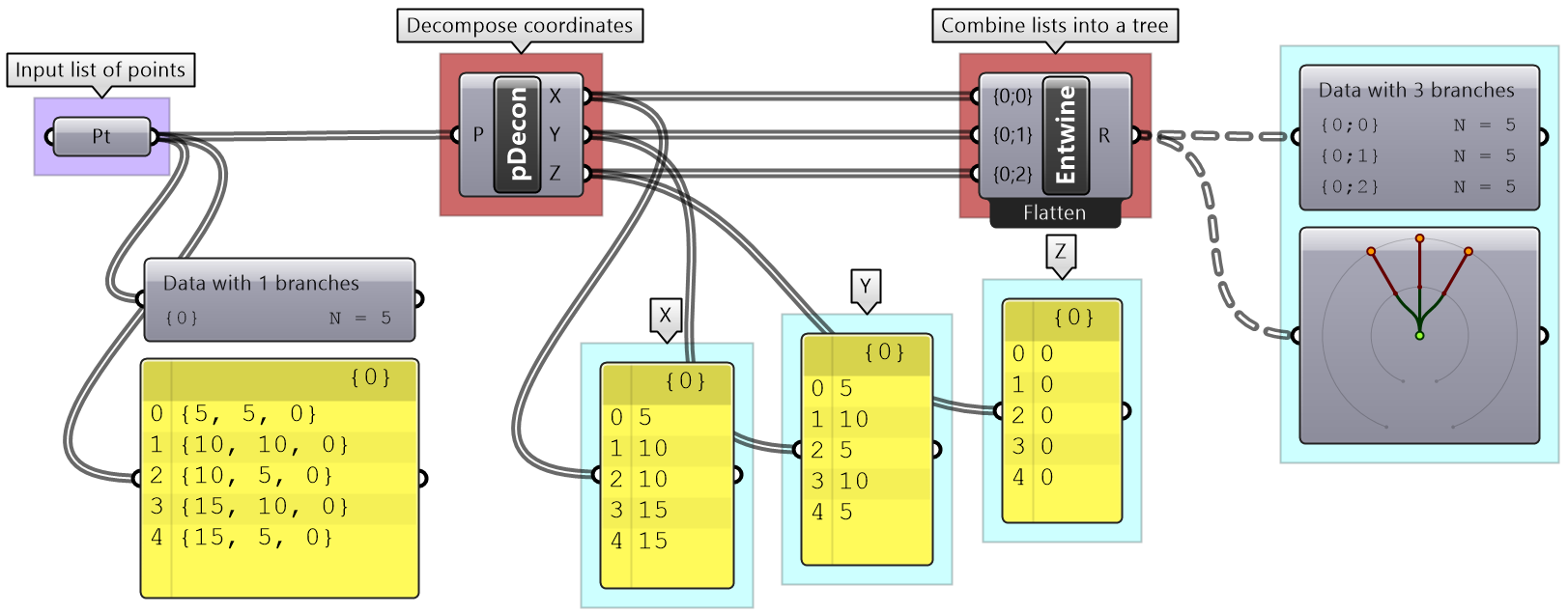

3.3 Tree matching

Matching data trees

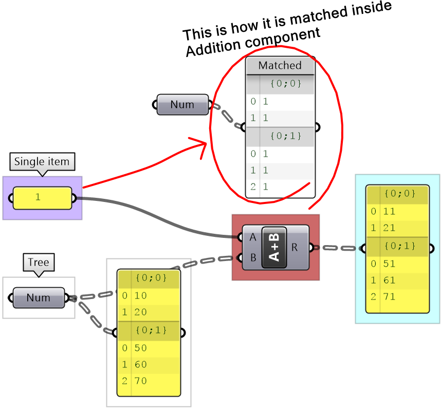
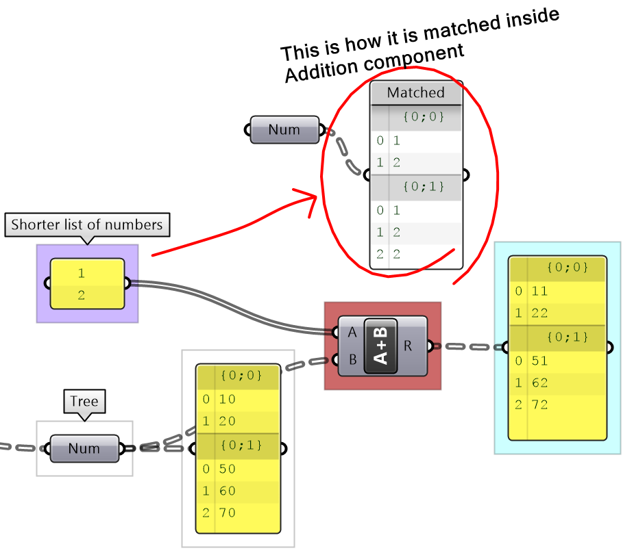
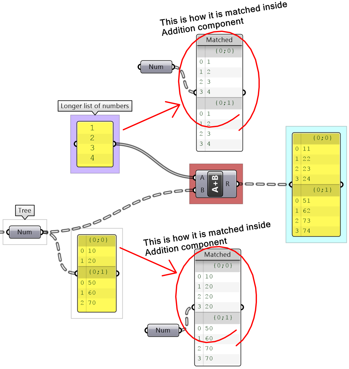
We explained the Long, Short and Cross matching with lists. Trees follow similar conventions to expand the shorter branches by repeating the last element to match. If one tree has fewer branches, the last branch is repeated. The following illustrates common tree matching cases.

3.3.1 Item-to-tree matching

When matching an item to a tree, a matching tree structure is created and the item is repeated. For example when adding a single number to a tree of numbers, the single number is added to every item in the tree and the result is a tree with matching structure to the input tree.

3.3.2 Short-list-to-tree matching

When matching a short list to a tree, where the length of the list is shorter than the tree branches, a matching tree structure is created where the list is repeated in each branch, and the last item in the short list is repeated. See the following example adding a list of two number to a tree of numbers.

3.3.3 Long-list-to-tree matching

When matching a long list to a tree with branches that are shorter than the list, the tree branches expand to match the length of the list. The last item in each branch is repeated to match the list length Note that the resulting tree structure will be differenent than the input tree. In the following example, both input, the list and the tree, are modified to arrive to a matching structure, then the addition result have than new data structure.

3.3.4 Tree-to-tree matching

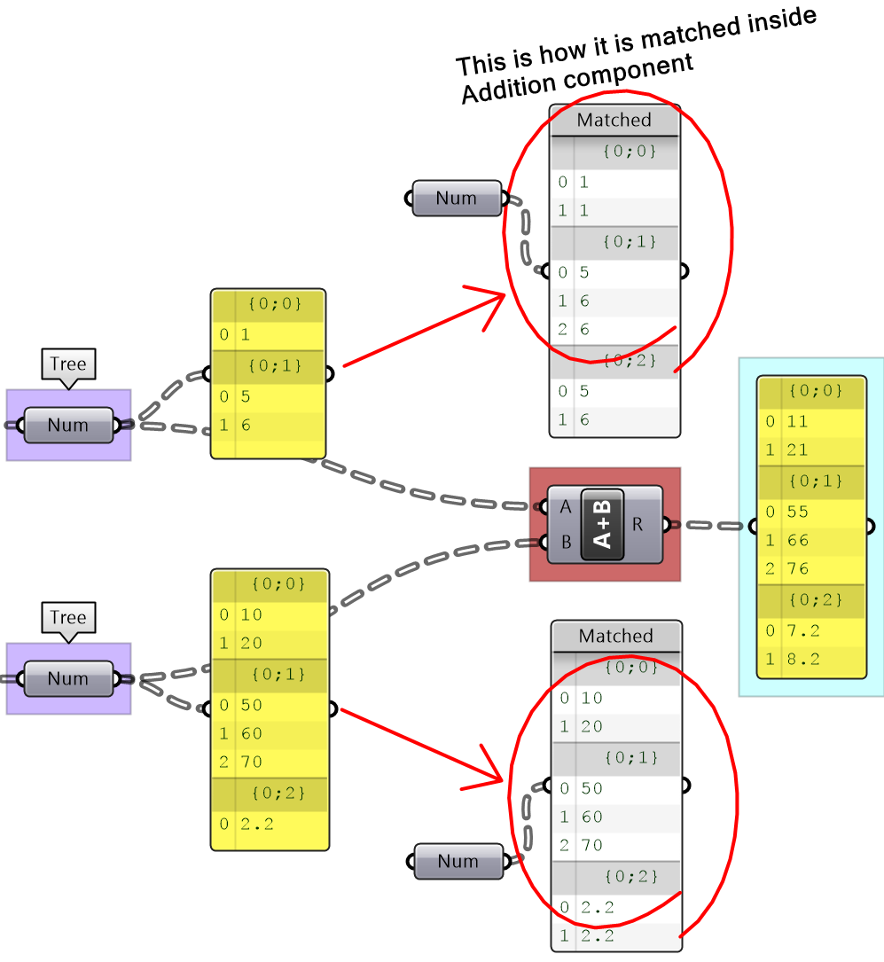
There are numerous possibilities when matching two trees, but the basic principle apply. The goal is to find a tree structure that can combine both input tree structure. Let’s assume the case when there is a simple tree with one level of branches that match in depth. There are two possibilities. The first is that both input trees have same number of branches. In this case, the length of the shorter corresponding branches is matched. The output tree might end up matching at least one of the input trees, or be different to both.

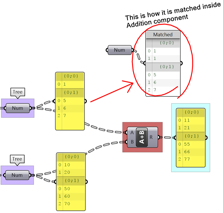
The second possibility is that one tree might have more branches than the other. In that case, new branches are inserted into the smaller tree repeating the last branch, then each branch is expanded (repeating the last item in the branch) to create matching length among all corresponding branches as in the following example.

When working with trees, it is of utmost importance to examine the data structure of each input before using it as input to one component. A small change in the structure can have big impact. For example, the following two trees of numbers appear to be matching at first, but because there is one level depth added to one of the trees (indicating an extra branch near the root of the tree), the result may be different than what is intended.

Tutorial 3.3.1 Tree matching
Inspect the following 2 number structures, then predict the structure and result of adding them (with default Grasshopper matching). Verify your answer using the Addition components.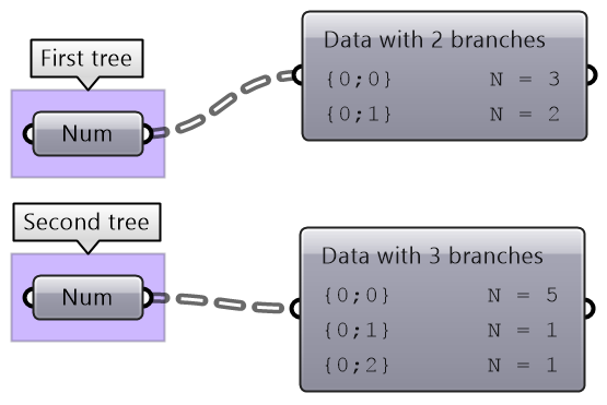
Solution... Key solution idea: The two input trees have different number of branches and different number of elements in each branch. The last branch of the shorter tree is repeated to match the number of branches, then corresponding branches are matched by repeating the last element of the shorter branch.

3.4 Traversing trees

Traversing data trees

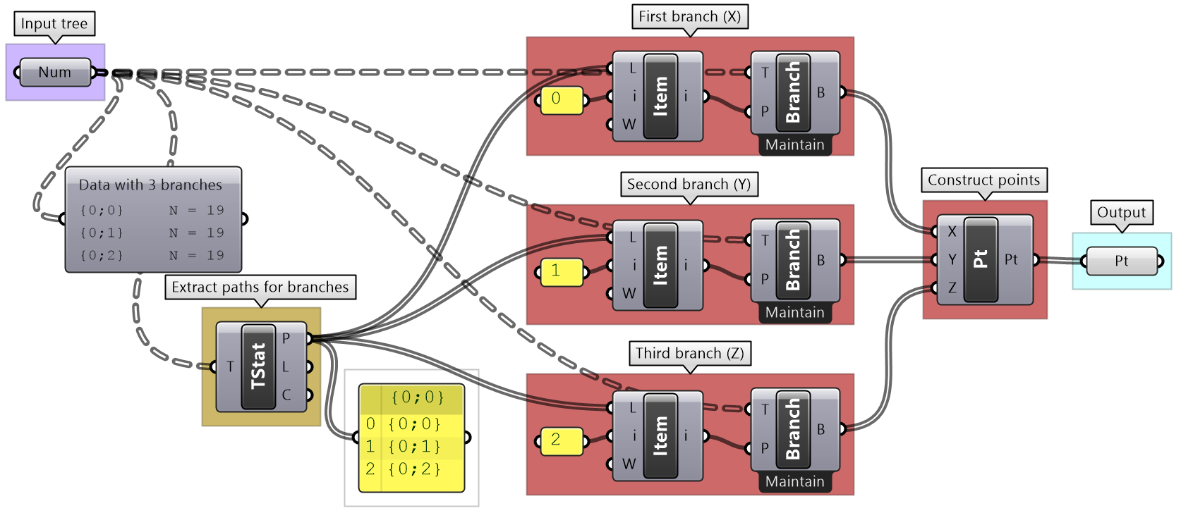
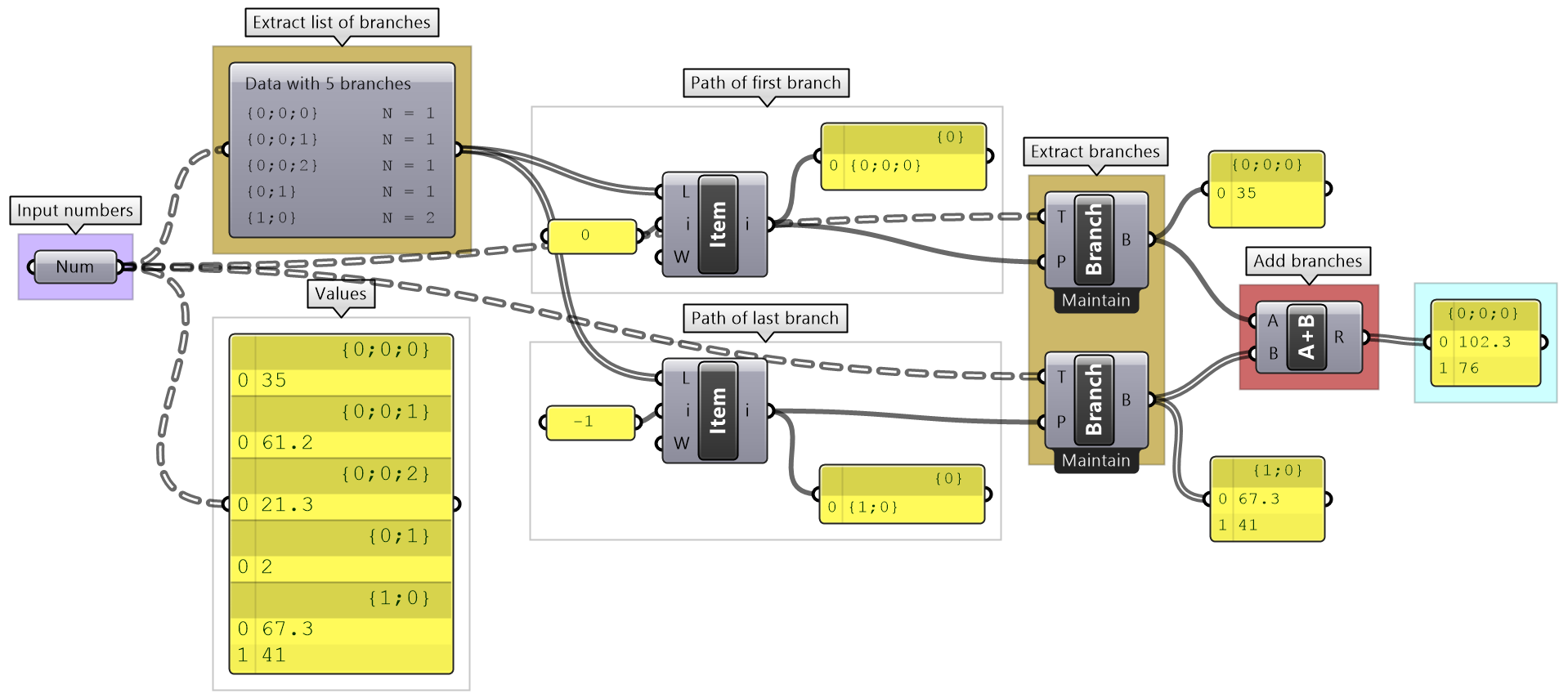
Grasshopper provides components to help extract branches and items from trees. If you have the path to a branch or to an item, then you can use Branch and Item components. You need to check the structure of your input so you can supply the correct path.

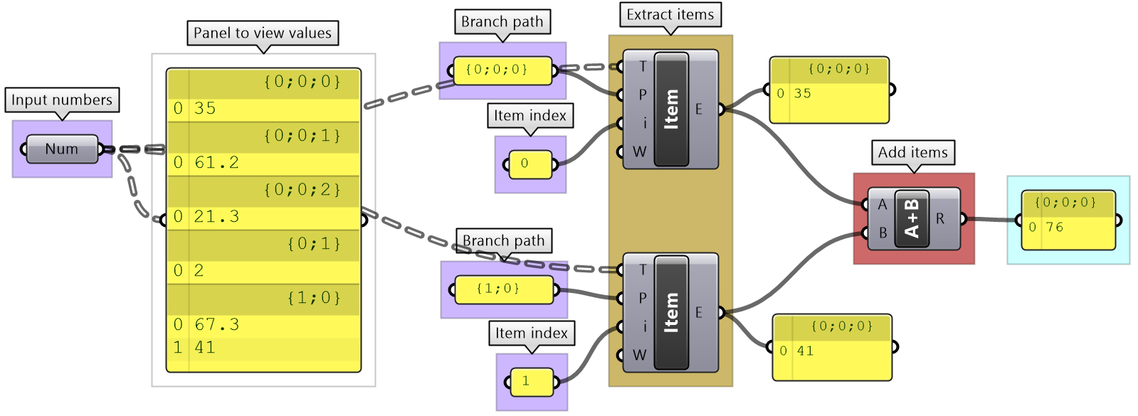
If you know that your structure might change, or you simply do not want to type the path, you can extract the path using the Param Viewer and List Item components.

Tutorial 3.4.1 Traversing trees
The following tree has 3 branches for each one of the coordinates (x, y, z) of some list of points. Use that tree to construct a list of these points.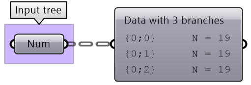
Solution... Key solution idea: We can construct a point list using as input 3 lists representing X, Y and Z values. If we can isolate the 3 branches of the input tree, then we will be able to feed them to the point construction component.

3.5 Basic tree operations

Basic tree operations are widely used and you will likely need them in most solutions. It is very important to understand what these operations do, and how they affect the output.

3.5.1: Viewing the tree structure

As we have seen in the data matching, different data structures of the same set of elements produce different results. Grasshopper offers three ways to view the data structure, the Parameter Viewer in text or diagram format, and the Panel.

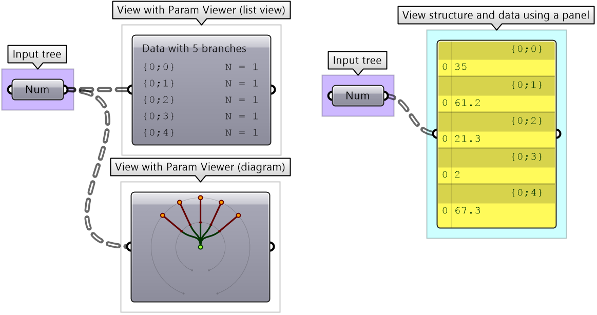
Tree information can be extracted using the TStats component. You can extract the list of paths to all branches, number of elements in each branch and the number of branches.

3.5.2 List operations on trees

List operations on data trees

Trees can be thought of as a list of branches. When using list operations on trees, each branch is treated as a separate list and the operation is applied to each branch independently. It is tricky to predict the resulting data structure and therefore it is always important to check your input and output structures before and after applying any operation. To illustrate how list operations work in trees, we will use a simple tree, a grid of points, and apply different list operations on it. We will then examine the output and its data structure.

Common list operation and how they apply to trees
List Item: Select items at specific index in each branch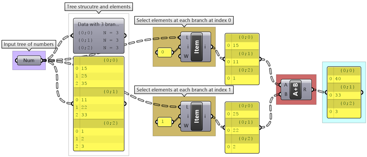
List Item: Select multiple indices to isolate part of the tree and perform one operation on such as Mass Addition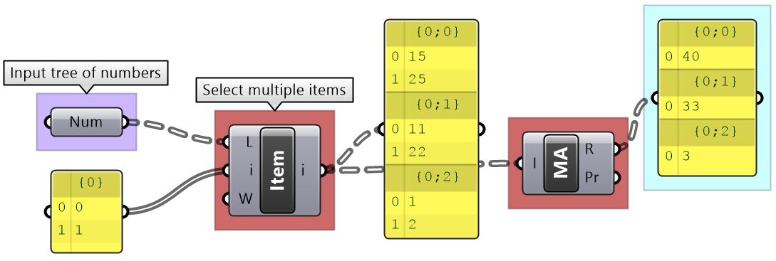
Split List: Split the elements of branches into 2 trees at the specified index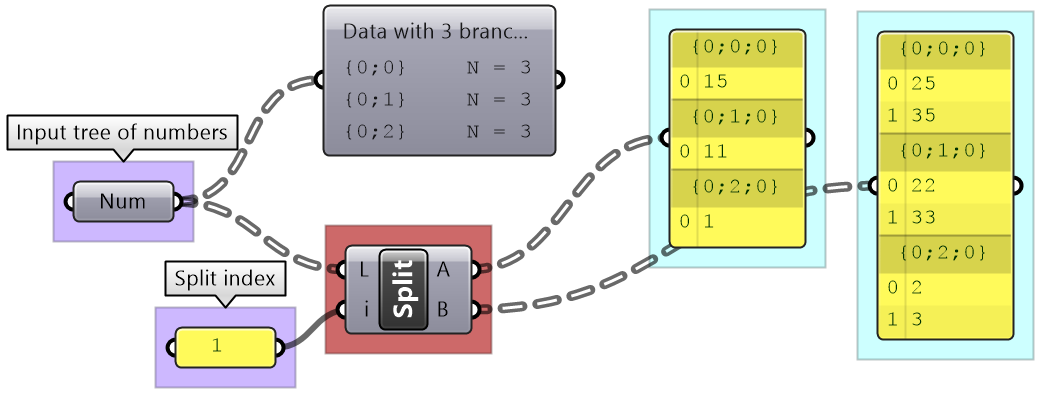
Shift List: Shifts the elements of each branch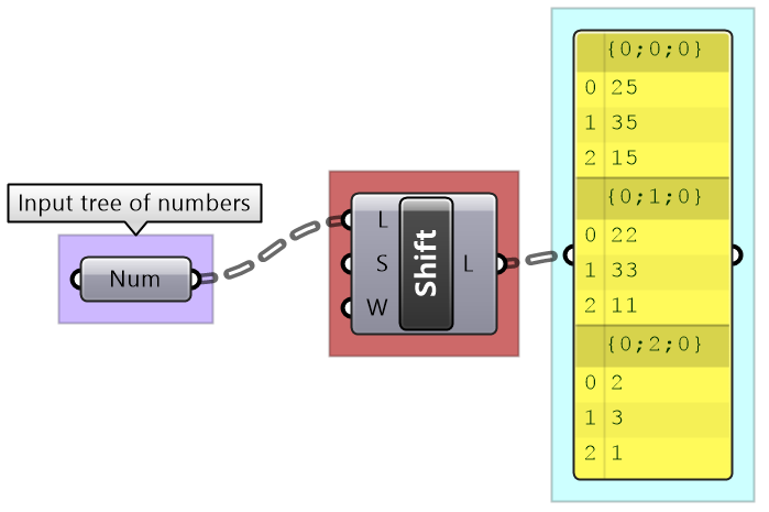
Cull Pattern: Culls each branch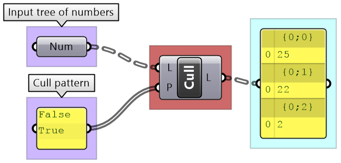

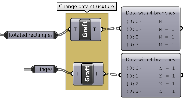
3.5.3 Grafting from lists to a trees

In some cases you need to turn a list into a tree where each element is placed in its own branch. Grafting can handle complex trees with branches of variable depths.

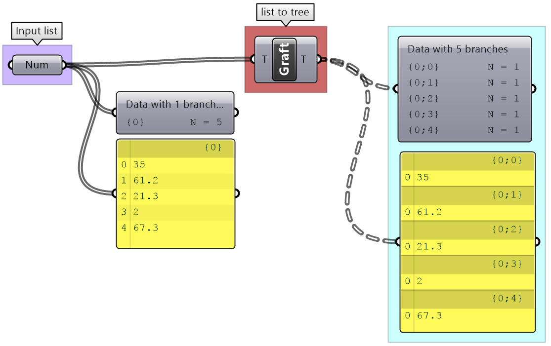
It might feel unintuitive to complicate the data structure (from a simple list to a tree), but grafting is very useful when trying to achieve certain matching. For example if you need to add each element of one list with all the elements in the second list, then you will need to graft the first list before inputting to the addition process.

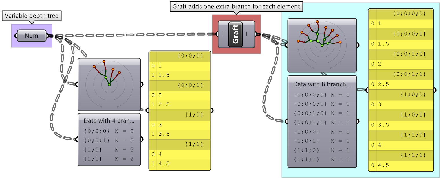
3.5.4 Flattening from trees to lists

Other times you might need to turn your tree structure into a simple list. This is achieved with the flattening process. Data from each branch is extracted and sequentially attached to one list.

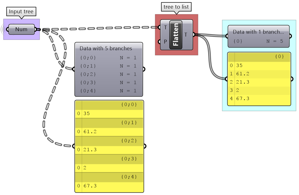
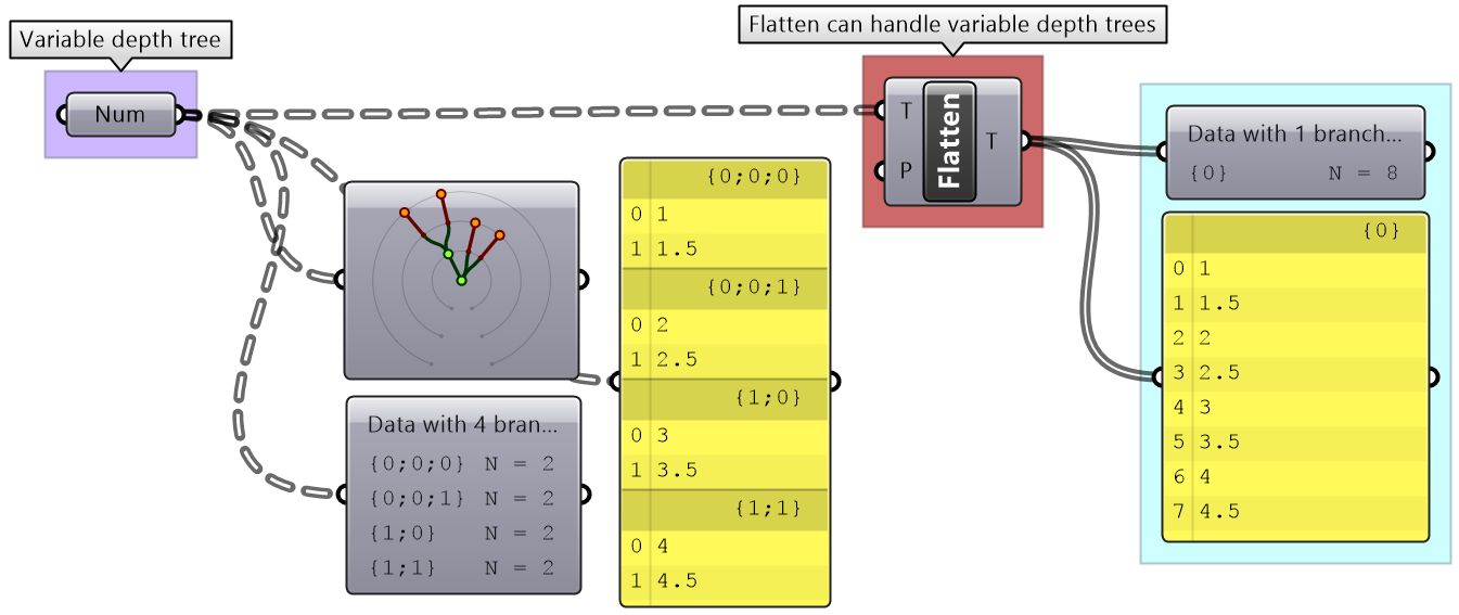
Flatten also can handle any complex tree. It takes the branches in order starting with the lowest index trunk and put all elements in one list.

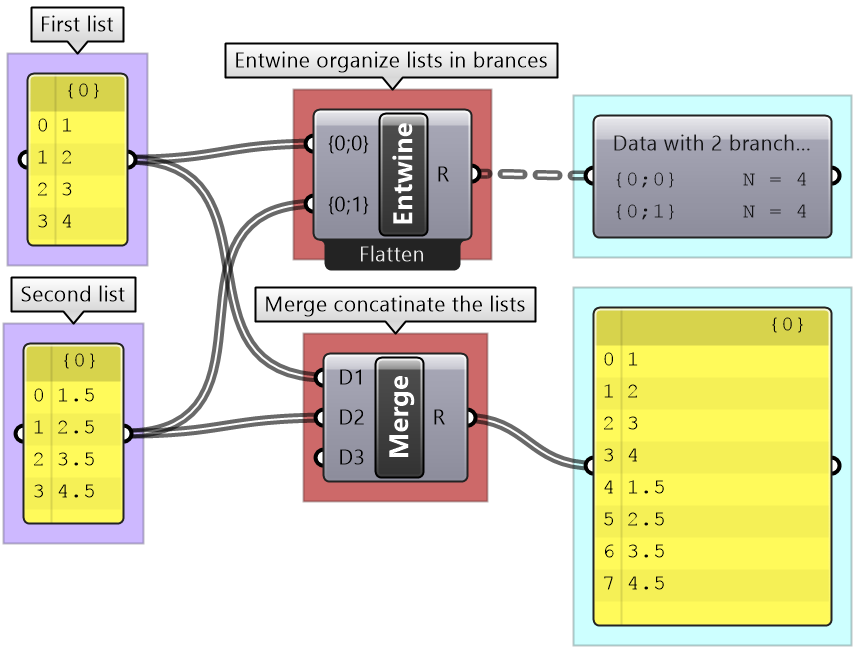
3.5.5 Combining data streams

It is possible to compose a number of lists into a tree where each list becomes a branch in a new tree. It is different from the merging of lists where simply one bigger list is created.

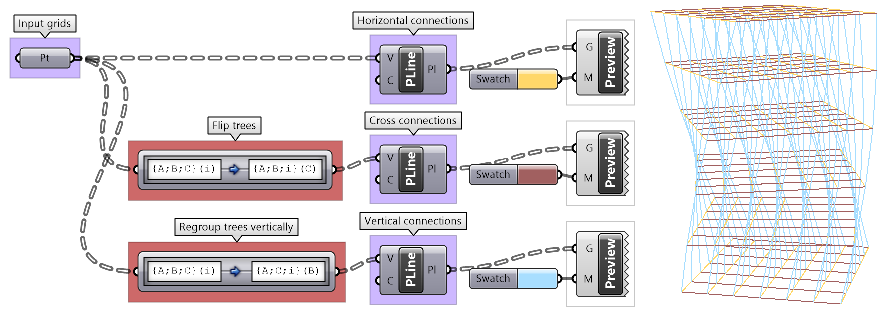
3.5.6 Flipping the data structure

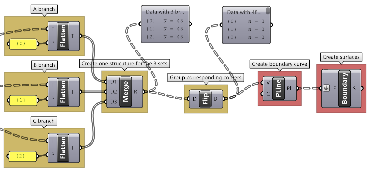
It is logical in some cases to flip the tree to change the direction of branches.This is specially useful in grids when points are organized in rows and columns (similar to a 2 dimensional array structure). Flipping causes corresponding elements across branches (have the same index in their branch) to be grouped in one branch. For example, a data tree that has 2 branches and 4 items in each branch, can be flipped into a tree with 4 branches and 2 elements in each branch.

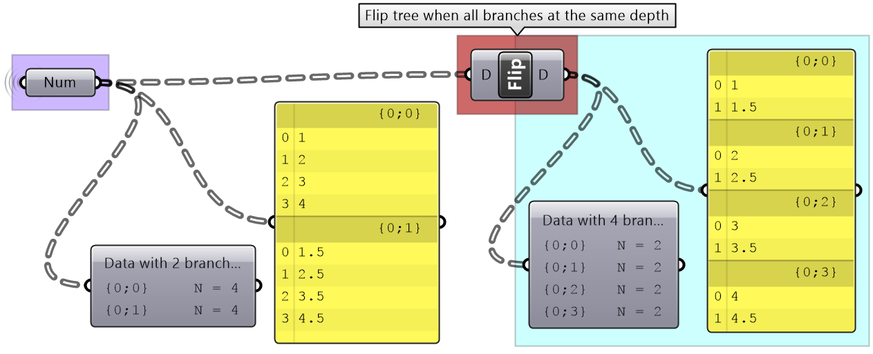
If the number of elements in the branches are variable in length, some of the branches in the flipped tree will have “null” values.

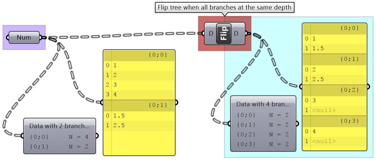
Flipping is one of the operations that cannot handle variable depth branches, simply because there is no logical solution to flip.

3.5.7 Simplifying the data structure

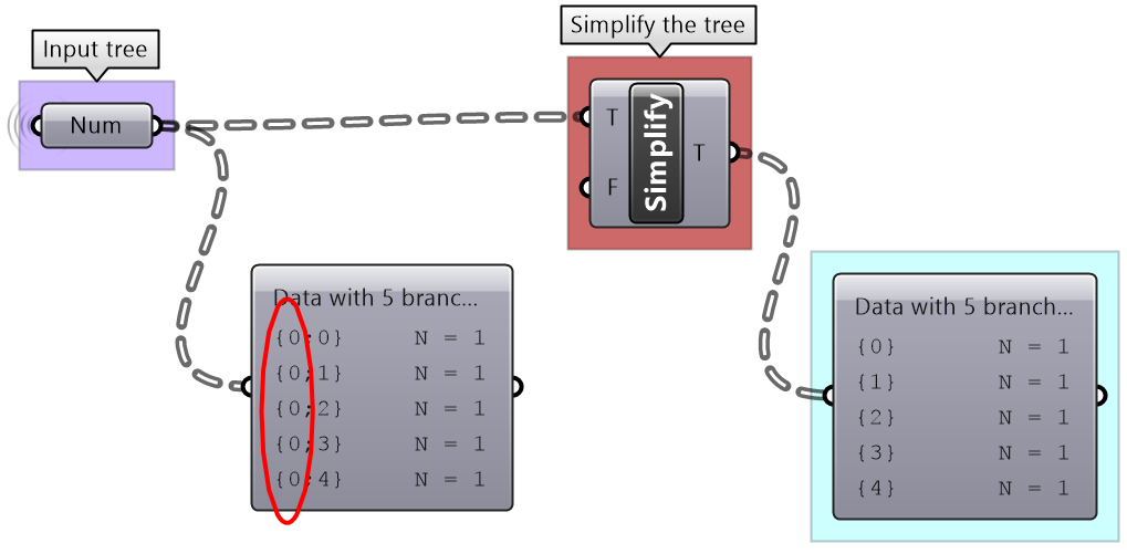
Processing data through multiple components can add unnecessary complexity to the data structure. The most common form is adding leading or trailing zeros to the paths addresses. Complex data structures are hard to match. Simplify Tree process helps remove empty branches. There are other operations such as Clean Tree and Trim Tree to help remove null elements, empty branches and reduce complexity. It is also possible to extract all branches as separate lists using the Explode Tree operation.

Tutorial 3.5.A Louvers
Given one curve on XY-Plane, create horizontal and vertical louvers as in the image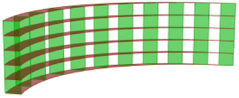
Solution... Examine the data structure of output from each step before feeding it into the next process: input curve data structure: Single item (one branch and one item in the branch) Divide input curve to extract points. Data structure: List (one branch with 11 items). Note that the path has added leading “0”. This indicates the next layer of calculation. Create vertical lines at each point. Data structure: List (one branch with 11 items). Note that the path did not increase in complexity. Divide vertical lines to create a grid of points. Data structure: Tree (11 branches with 6 items). Note that the path has added leading “0”. Create horizontal lines at each point. Data structure: Tree (11 branches with 6 items). Note that the path did not increase in complexity. Create lofted surfaces through branches of lines. Data structure:Tree (11 branches with 1 item each). Note that the path did not increase in complexity. Flip the tree matrix and then create lofted surfaces through branches of lines. Data structure: Tree (11 branches with 1 item each). Note that the path did not increase in complexity. You can flatten the tree to create one list of horizontal louvers.

Tutorial 3.5.B Shutters
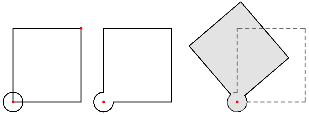
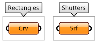
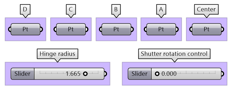
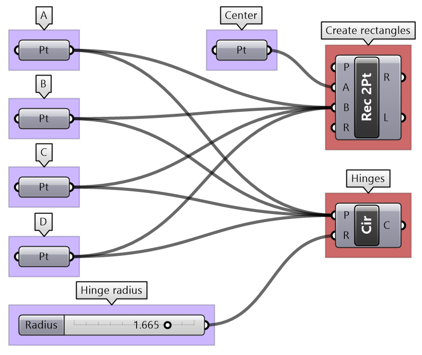
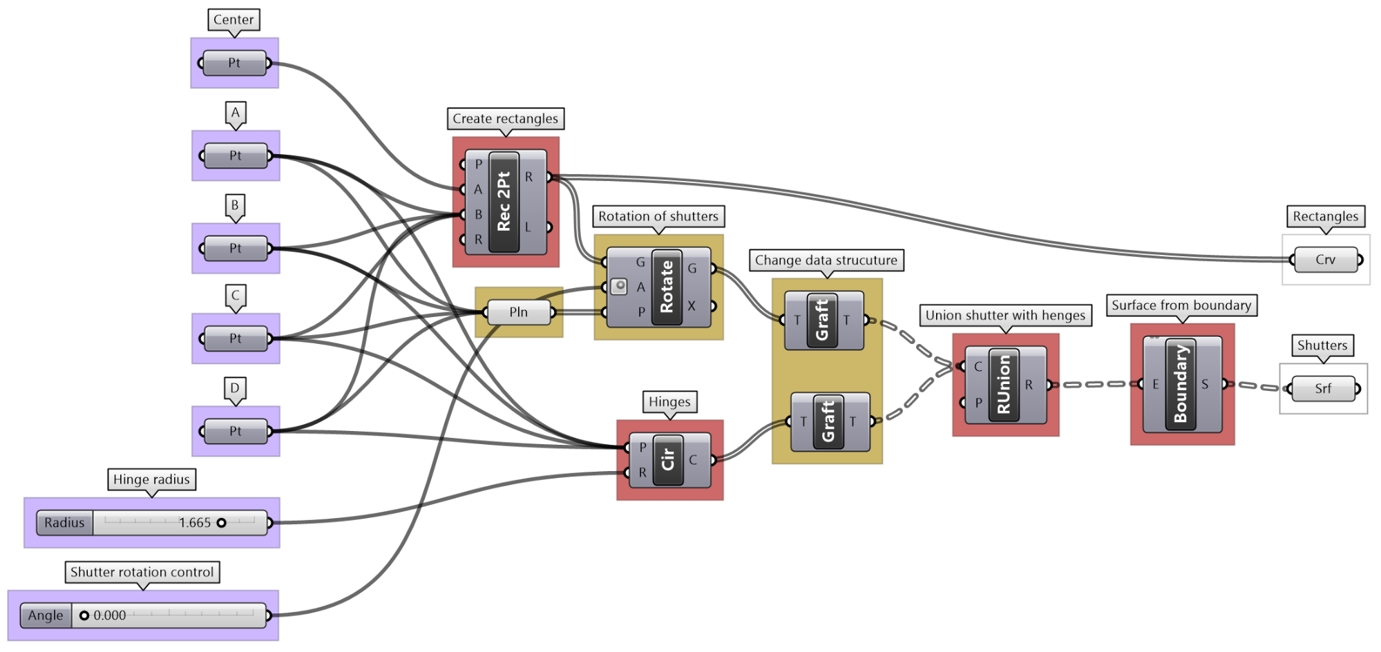
Given four corner points on a plane and a radius for the hinge, create a shutter that can open and shut as in the image using a rotation parameter
Solution... Algorithm analysis: For each shutter there are two parts: the rectangle and the hinge. Union the rectangle and hinge, then allow rotating around the hinge. There is one rotation control to move all shutters together. Solution steps: Output: Surface of the shutters and curves for the frame Input: The window four corner points (and center), the hinge radius and the rotation angle parameter Key processe #1: create rectangle and hinges. Use the Rectangle component Key processe #2: Union the curves. Use the RUnion component, then create a surface from the boundary using Boundary component Intermediate process #1: Rotate the rectangles using the angle. Use Rotate component Properly match the data structures of the rectangles and hinges before the region union. Use the Graft so that rectangles and hinges pair correctly. Putting it all together:

3.6 Advanced tree operations

As your solutions increase in complexity, so will your data structures. We will discuss three advanced tree operations that are necessary to solve specific problems, or are used to simplify your solution by tabbing directly into the power of the data tree structure.

3.6.1 Relative items

Advanced data trees operations: Relative item

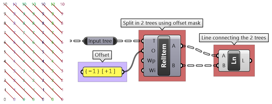
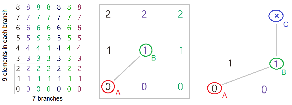
The first operation has to do with solving the general problem of connectivity between elements in one tree or across multiple trees. Suppose you have a grid of points and you need to connect the points diagonally. For each point, you connect to another in the +1 branch and +1 index. For example a point in branch {0}, index [0], connects to the point in branch {1}, index [1].

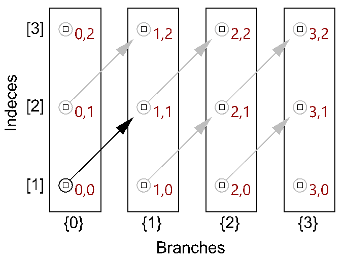
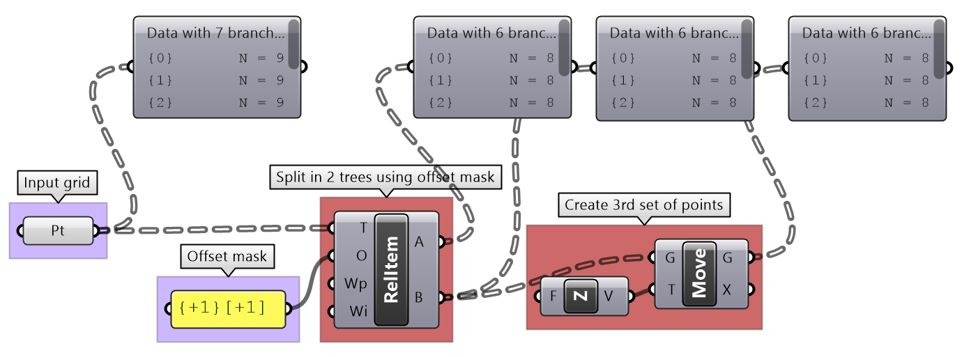
In Grasshopper, the way you communicate the offset is expressed with an offset string in the format “{branch offset}[index offset]”. In our example, the string to connect points diagonally is “{+1}[+1]”. Here is an example that uses relative tree component in Grasshopper. Notice that the relative item component creates two new trees that correlate in the manner specified in the offset string.

Here is an example implementation in Grasshopper where we define relative items in one tree, then connect the two resulting trees with lines using the Relative Item component.

Tutorial 3.6.1.A Relative item pattern
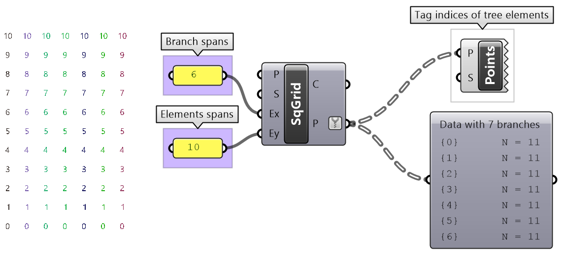
Create the pattern shown in the image using a square grid of 7 branches where each branch has11 elements.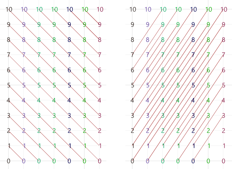
Solution... Create the grid Create relative trees that connect each element with -1 branch and +1 index: {-1}[+1] Create lines to connect the 2 relative trees. Change the offset to {+2}[+3] to create the second connections

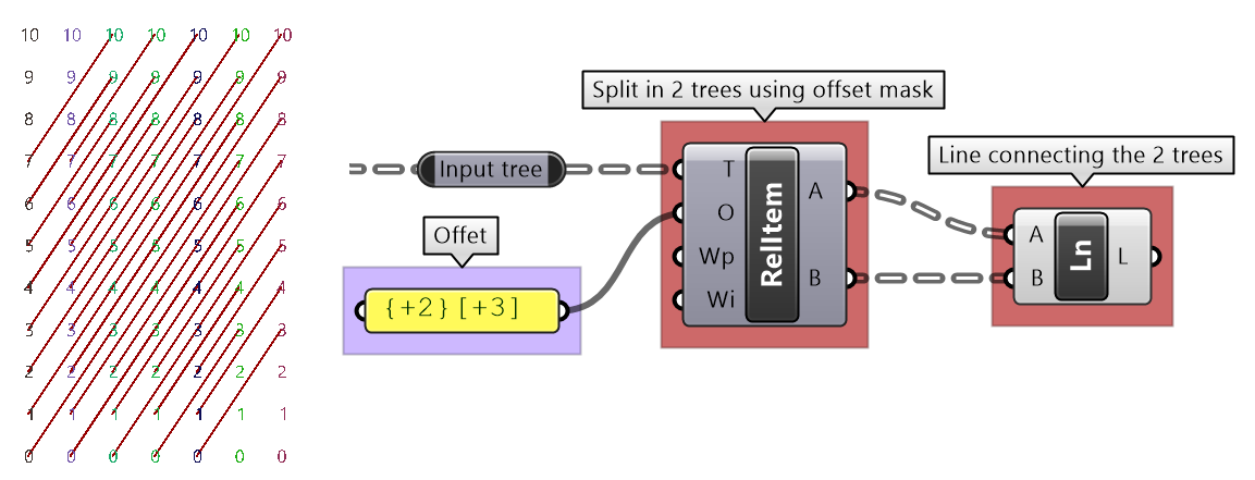
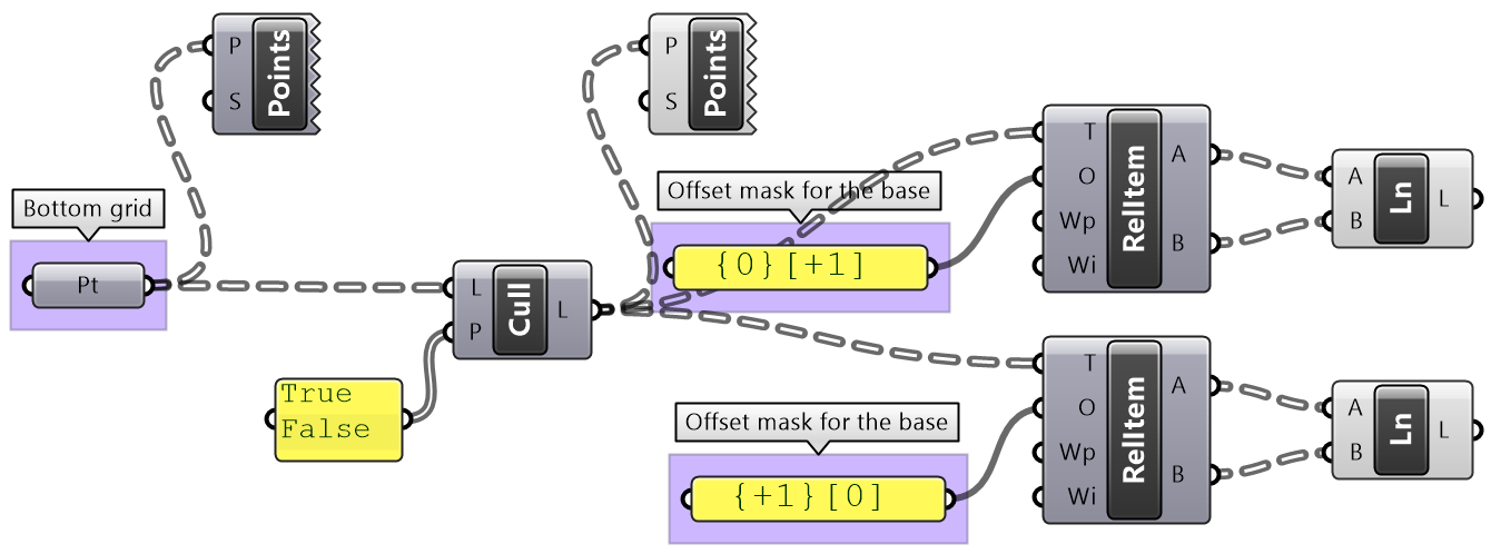
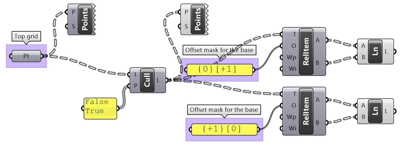
We showed how to define relative items in one tree, but you can also specify relative items between 2 trees. You’ll need to pay attention to the data structure of the two input trees and make sure they are compatible. For example, if you connect each point from the first tree with another point from a different tree with the same index, but +1 branch, then you can set the offset string to be {+1}[0].

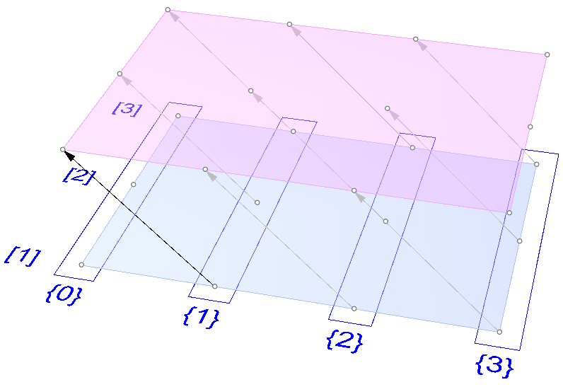
The input to the Relative Items component is two trees and the output is two trees with corresponding items according to the offset string.

The following GH definition achieves the above:

Tutorial 3.6.1.B Relative item truss
Use relative items between 2 bounding grids to generate the structure shown in the image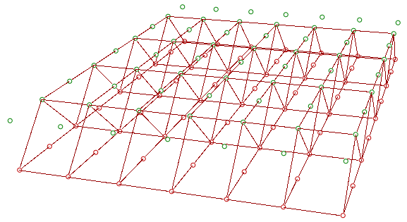
Solution... Solution video... Create the connections for the bottom tree Cull every other index and keep the same number of branches (cull indices 1, 3,...) Define the offset strings for RelativeItem components to create the vertical and horizontal connections The Grasshopper definition: Create the connections for the top tree Cull every other index and keep the same number of branches. (cull indices 0, 2,...) Define the offset strings for RelativeItem components to create the vertical and horizontal connections The Grasshopper definition: Connections between the bottom and top trees Use culled grids, then define first offset string for RelativeItems component to create the first set of cross lines: {0}[0] Define second offset string for RelativeItems component to define the second set of cross lines: {0}[-1]

3.6.2 Split trees

Split data trees

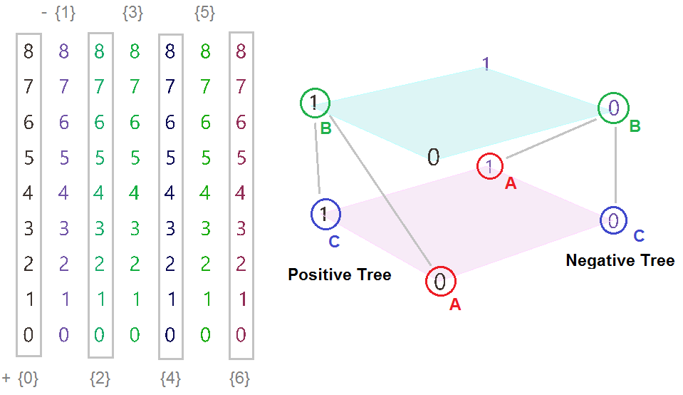
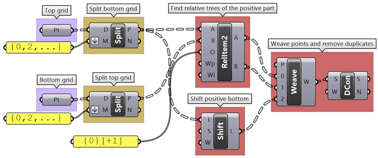
The ability to select a portion of a tree, or split into two parts is a very powerful tree operation in Grasshopper. You can split the tree using a string mask using specific syntax (see examples below). The mask filters, or helps select, the positive part of your tree. The portion of the tree left, is also given as an output and is called the negative part of the tree. Since all trees are made out of branches and indices, the split mask should include information about which branches and indices within these branches to split along. Here are the rules of the split mask:

Mask syntax	General rules
{ ; ; }	Use curly brackets to enclose the mask for the tree branches.
[ ]	Use square brackets to enclose the mask for the elements (leaves). Can be omitted if select all items or use [*]
( )	Round brackets are used for organizing and grouping
*	Any number of integers in a path. The asterisk also allows you to include all branches, no matter what their paths look like
?	Any single integer
6	Any specific integer
!6	Anything except a specific integer
(2,6,7)	Any one of the specific integers in this group.
!(2,6,7)	Anything except one of the integers in this group.
(2 to 20)	Any integer in this range (including both 2 and 20).
!(2 to 20)	Any integer outside of this range.
(0,2,...)	Any integer part of this infinite sequence. Sequences have to be at least two integers long, and every subsequent integer has to be bigger than the previous one (sorry, that may be a temporary limitation, don't know yet).
(0,2,...,48)	Any integer part of this finite sequence. You can optionally provide a single sequence limit after the three dots
!(3,5,...)	Any integer not part of this infinite sequence. The sequence doesn't extend to the left, only towards the right. So this rule would select the numbers 0, 1, 2, 4, 6, 8, 10, 12 and all remaining even numbers.
!(7,10,21,...,425)	Any integer not part of this finite sequence.
{ * }[ (0 to 4) or (6,11,41) ]	It is possible to combine two or more rules using the boolean and/or operators. The example selects the first five items in every list of a tree and also the items 7, 12 and 42.

Here are some examples of valid split masks.

Split mask by branches	Description
{ * }	Select all (the whole tree output as positive, and negative tree will be empty)
{ *; 2 }	Select the third branch
{ *; (0,1) }	Select the first two end branches
{ *; (0, 2, …) }	Select all even branches

Split mask by branches and leaves	Description
{ * }[(1,3,...)]	Select elements located at odd indices in all branches
{ *; 0 }[(1,3,...)]	Select elements located at odd indices in the first branch
{ *; (0, 2) }[(1,3,...)]	Select elements located at odd indices in the first and third branches
{*; (0,2,...) } [ (1,3,...) ]	Select elements located at odd indices in branches located at even indices
{*; (0,2,...) } [(0) or (1,3,...)]	Select elements located at odd indices, and index “0”, in branches located at even indices

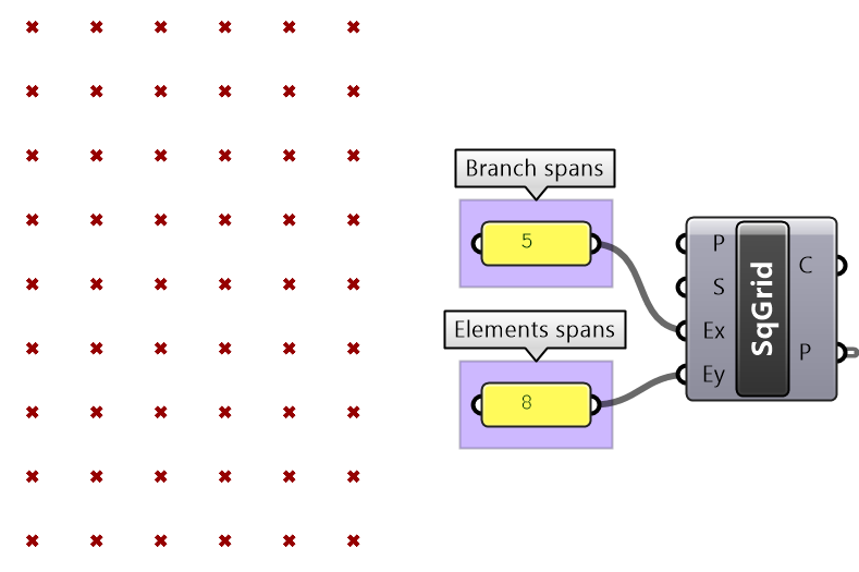
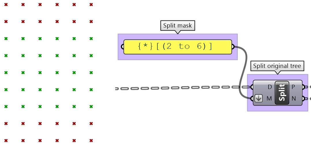
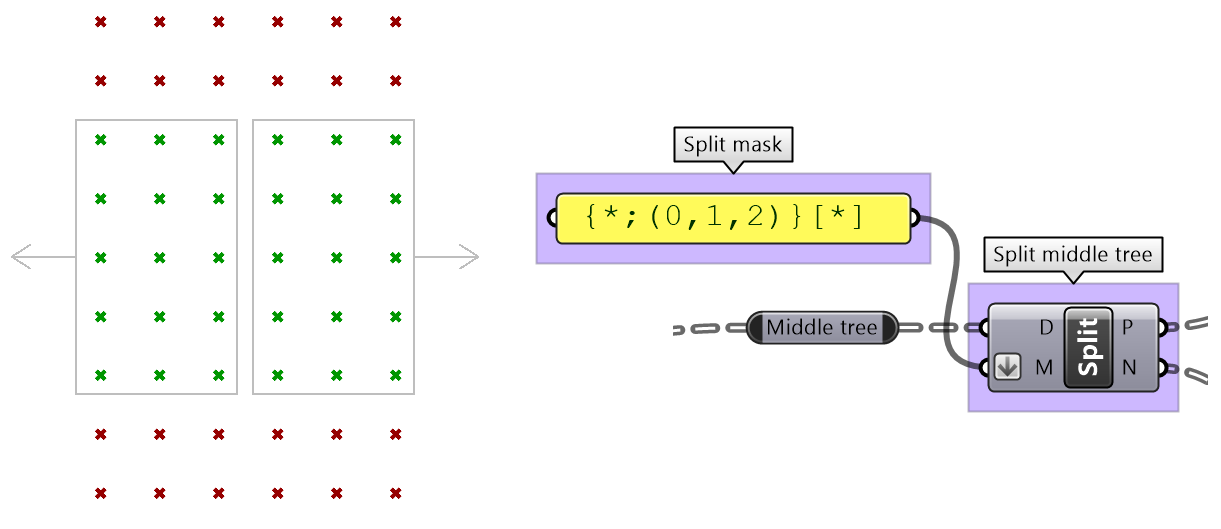
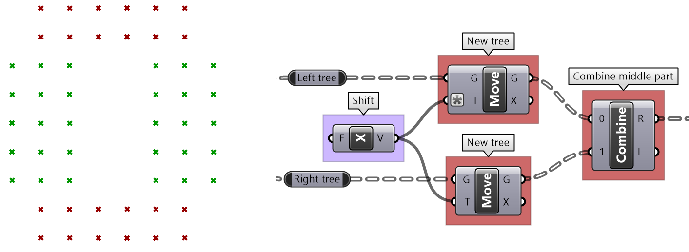
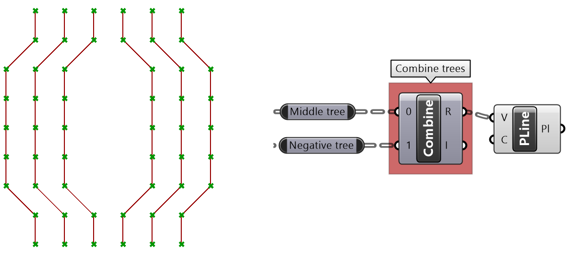
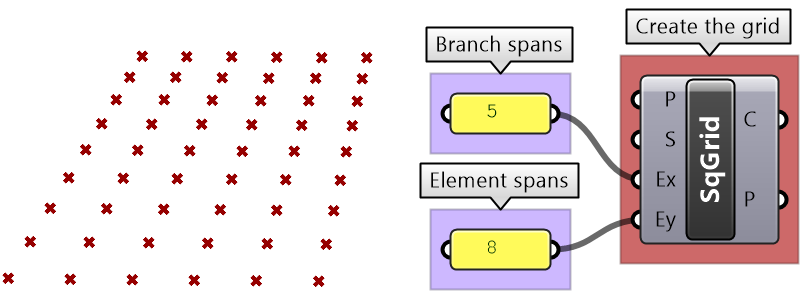
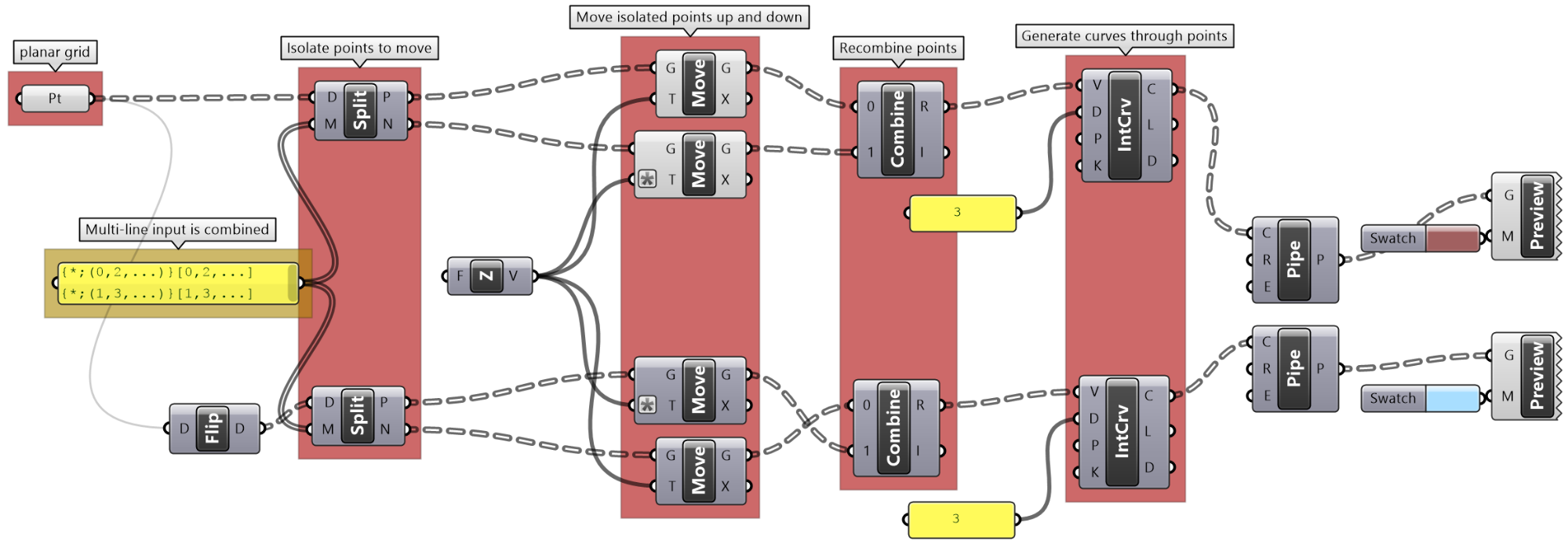
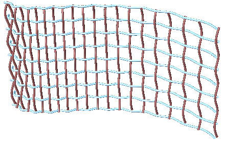
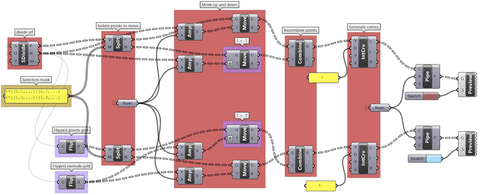
One of the common applications that uses split tree functionality is when you have a grid of points that you like to transform a subset of. When splitting, the structure of the original tree is preserved, and the elements that are split out are replaced with null. Therefore, when applying transformation to the split tree, it is easy to recombine back. Suppose you have a grid with 7 branches and 11 elements in each branch, and you’d like to shift elements between indices 1-3 and 7-9. You can use the split tree to help isolate the points you need to move using the mask: {*}[ (1,2,3) or (7,8,9) ], move the positive tree, then recombine back with the negative tree.

This is the GH definition that does the above using the Split Tree component.

One of the advantages of using Split Tree over relative trees is that the split mask is very versatile and it is easier to isolate the desired portion of the tree. Also the data structure is preserved across the negative and positive trees which makes it easy to recombine the elements of the tree after processing the parts.

Tutorial 3.6.2.A: Split tree pattern
Given a 6x9 grid, use the split tree to generate the following pattern: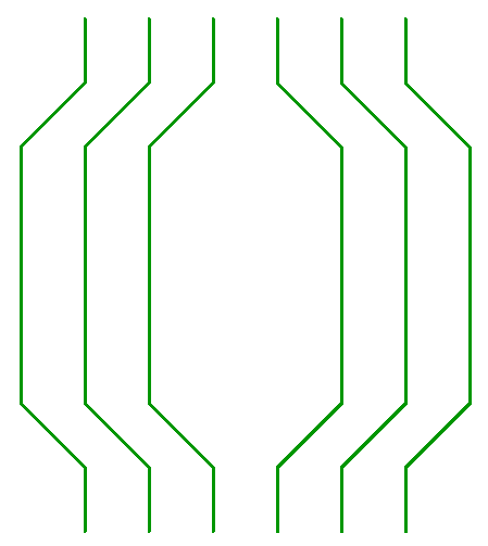
Solution... Create the grid Split the tree to isolate the middle part Split the middle part into two new parts Move the two middle parts in opposite directions then recombine them Recombine the middle part with the rest of the tree and create polylines through each branch elements

Tutorial 3.6.2.B: Split tree truss
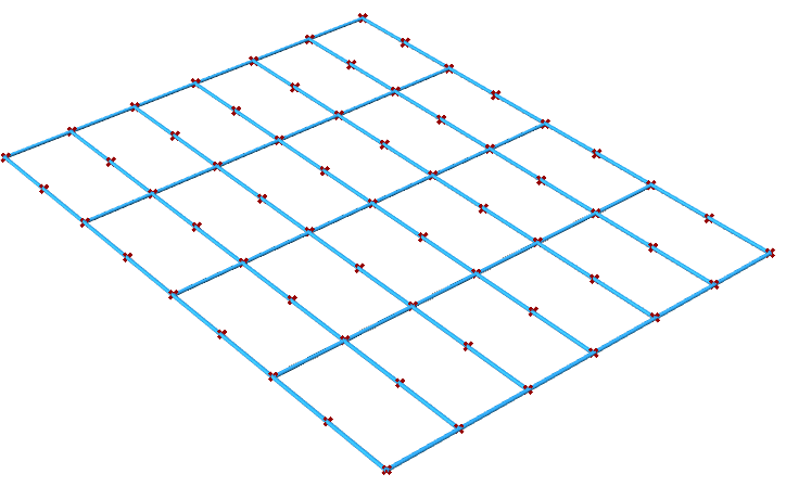
Given a grid, create the following truss system using the split tree method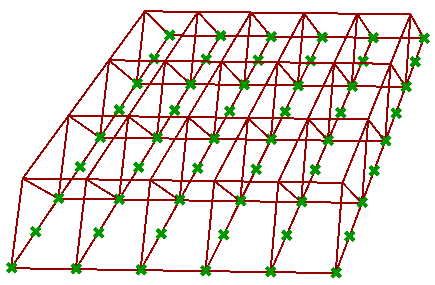
Solution... Solution video... Create the 6x9 grid Split at every other element Move positive tree vertically Combine positive and negative trees, and create a polyline through each branch Create bottom curves using negative tree Create top curves using positive tree

3.6.3 Path mapper

Why use the Path Mapper?
Syntax of the Path Mapper

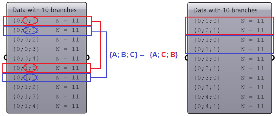
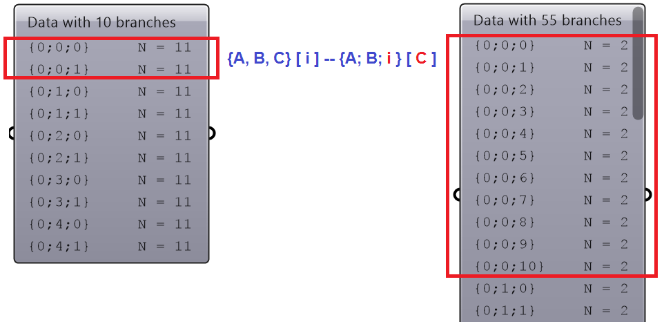
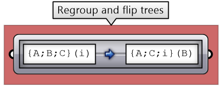
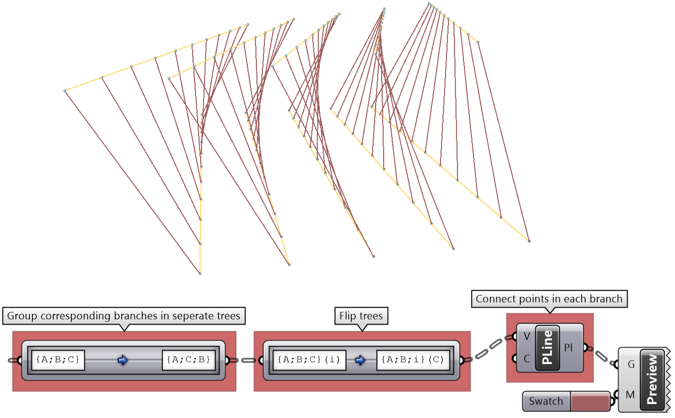
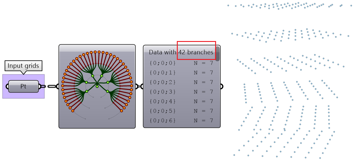
When dealing with complex data structures such as the Grasshopper data trees, you’ll find that you need to simplify or rearrange your elements within the tree. There are a few components offered in Grasshopper for that purpose such as Flatten, Graft or Flip. While very useful, these might not suffice when operating on multiple trees or needing custom rearrangement. There is one very powerful component in Grasshopper that helps with reorganizing elements in trees or change the tree structure called the Path Mapper. It is perhaps the least intuitive to use and can cause a loss of data, but it is also the only way to find a solution in some cases, and hence it pays to address here. The Path Mapper maps data between source and target paths. The source path is fixed, and is given by the input tree. You can only set the target path. There is a set of constants that you can use to help construct the mapping. Those are listed in the table below.

Path Mapper Constants	Description
item_count	Number of items in the current branch
path_count	Number of paths (branches) in the tree
path_index	Index of the current path

Let’s start by familiarizing ourselves with the syntax using built-in mappings inside the Path Mappers. If you right-muse-click on the mapper components, you can open the editor, and also access a bumber of default mapping functions that are commonely used.

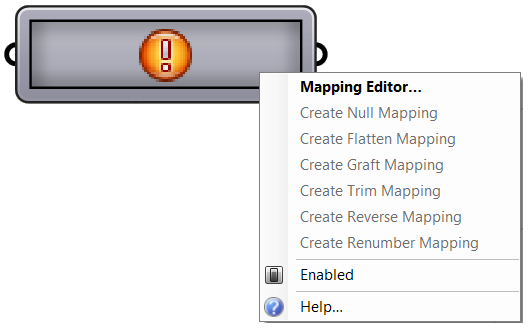
The Null Mapping does not change the data tree organization, but it offers a good start because it populates the editor with the input data structure. Set the mapping to Null Mapping and double click on the component to open the editor. The default tree source include the path only to start, but can add the data index part if needed for your mapping.

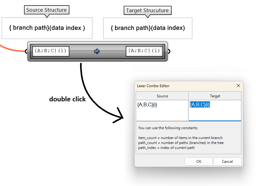
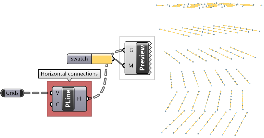
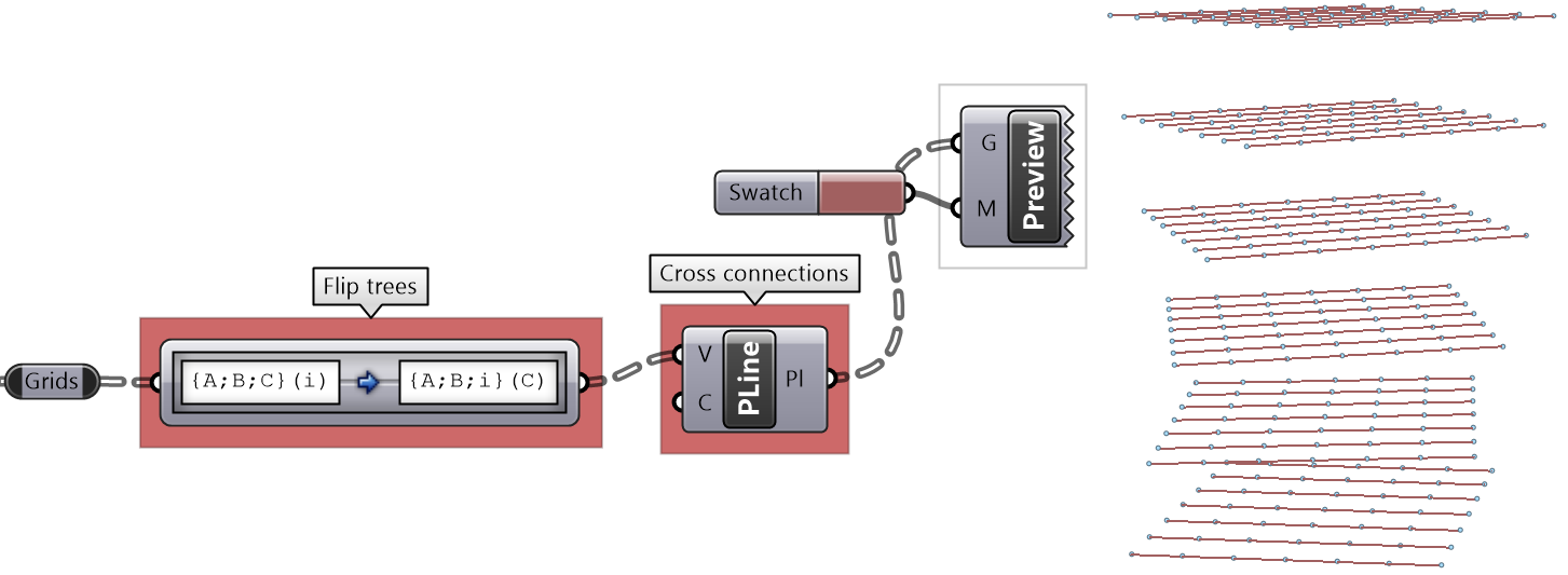
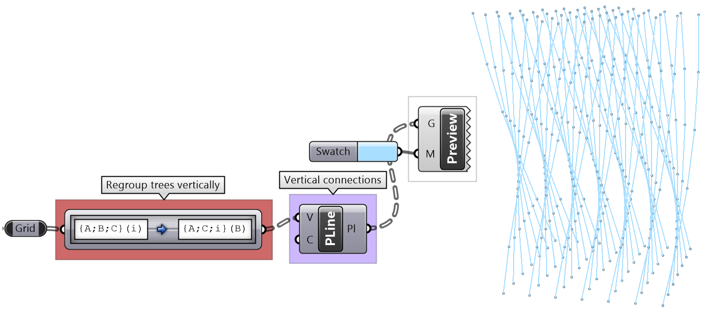
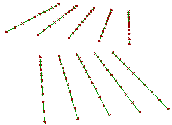
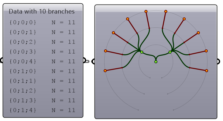
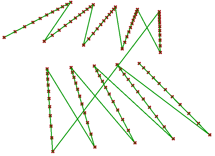
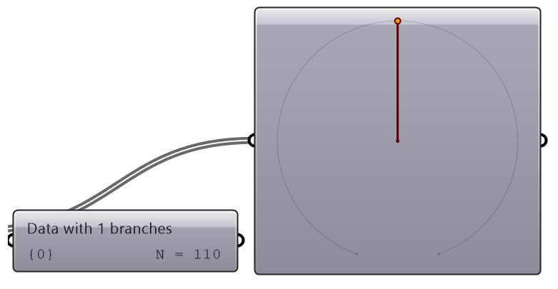
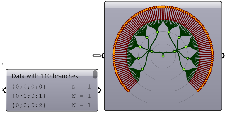
The following example examines different built-in mapping in the Path Mapper and how it changes the data structure. The Polyline component creates one polyline through each branch of the tree. Notice how different mapping affect the result.

Mappings
Null	Output = Input tree
Flatten	Convert to a list
Graft	Put leaves in branches
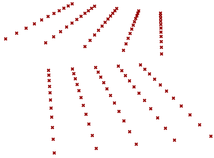Reverse	Reverse the tree
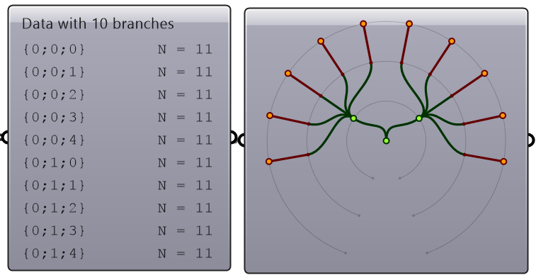Renumbering	Renumber branches

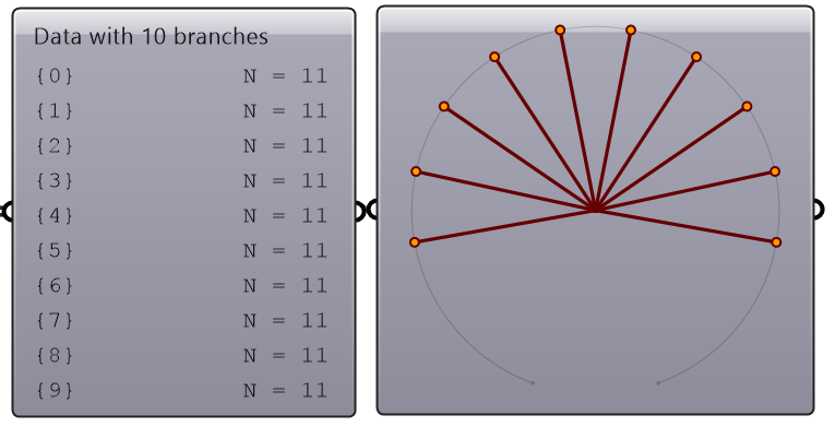For more details about the Path Mapper, please refer to the help inside the component in Grasshopper.

Tutorial 3.6.3.A: Partitions
Given a grid, create the following truss system using the split tree method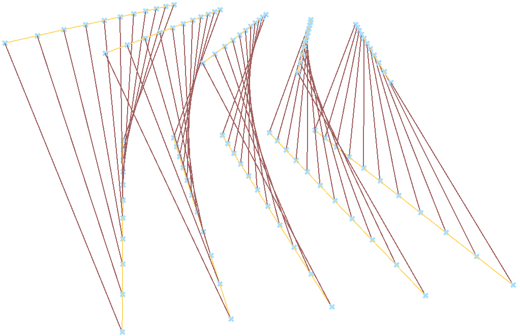
Solution... The input has two trees, and each has 5 branches with 11 elements in each branch, a total of 10 branches A Polyline is used to connect the elements in each branch To create the vertical connections, you need to create a branch for each 2 corresponding elements across the 2 trees, then use Polyline to connect them 1. Analyze the paths of the trees 2. Come up with a mapping that generates the desired grouping First, group corresponding branches across the 2 trees. That can be achieved by switching the last two integers in the paths: Second, Flip each of the 5 trees. Since the branches have 11 elements each, flipping each tree will create 11 branches with 2 elements in each branch. Total of 55 branches. You flip by switching the last integer of the path with the element index: Finally, a Polyline makes the vertical connections. Note: You can combine the 2 mappings in one step as in the following:

Tutorial 3.6.3.B: Bruilding structure
Given the input tree of points, create the following structure.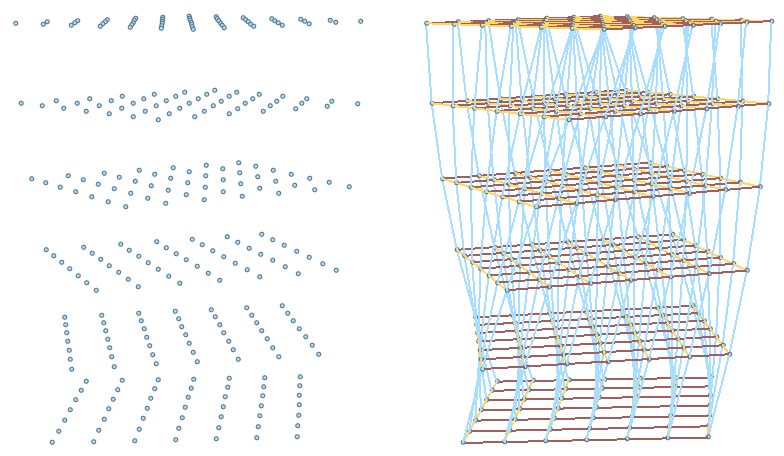
Solution... The initial tree has 42 branches, 7 branches in each of the 6 trees The Polyline component connects the elements in each branch Flip the trees using Path Mapper by switching branch and element indices Regroup the elements of corresponding branches in all trees using the Path Mapper Final result Create all connections

3.7 Tutorials: advanced data structures

Tutorial 3.7.1: Sloped roof
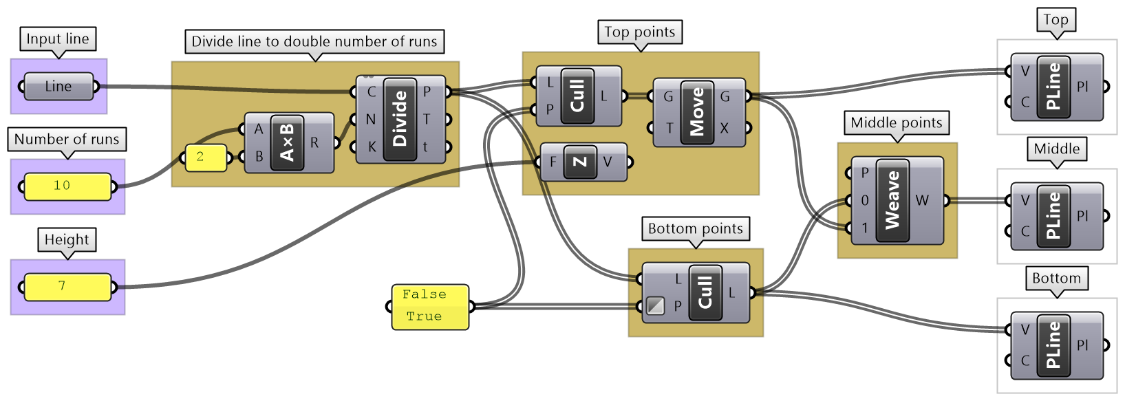
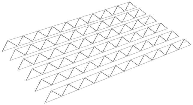
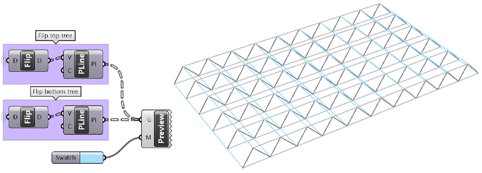
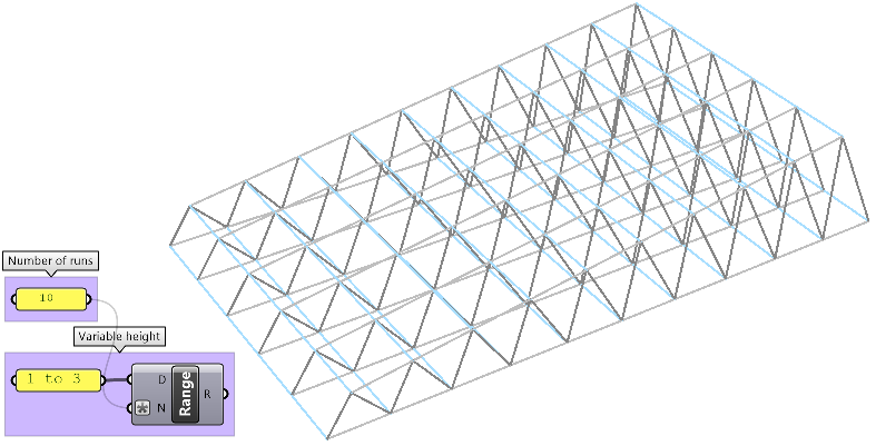
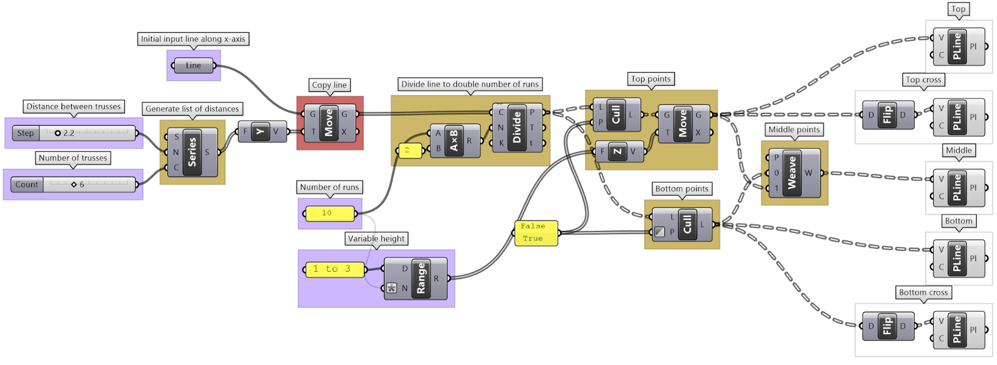
Create a parametric truss system that changes gradually in height as shown in the image.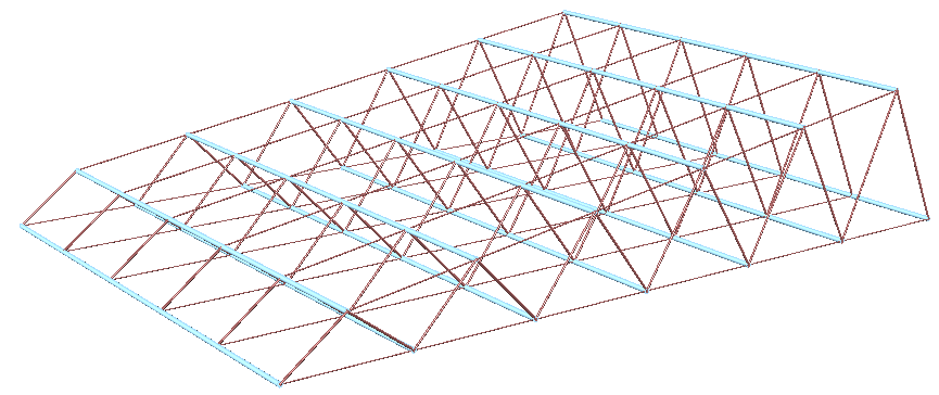
Solution... ownload GH file... Algorithm analysis: First, solve it for one simple truss Identify desired output for a single truss Define initial input 1- Base line on XY-Plane 2- Number of runs 3- Height Algorithms steps: Create input (L=line, H=height and R= #runs) Divide curve by 2*R Move every other point in the Z direction by height Create 3 sets of ordered points for the bottom beams, top beams and middle beams, then connect each of the 3 sets with a polyline Implement the algorithm for a single truss In Grasshopper: Resolve for multiple trusses with variable height: Create a series of base lines using the initial line and copy in Y-Axis direction Use the list of lines as input instead of a single line. Notice that instead of a list of points for each of the 3 sets (bottom, top and middle), we now have a tree or grid of points with a number of branches equal to the number of trusses Create cross connections using Flip tree operation for the bottom and top trees Create variable height The complete solution implementation in Grasshopper:

Tutorial 3.7.2: Diagonal triangles
Given the input grid, use the RelativeItem component to create diagonal triangles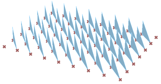
Solution... download GH file... Algorithm analysis: To generate the triangles, we need 3 sets of corner points. Two of the point sets (A, B) are within the grid. B is diagonal from A (relative index is +1 branch and +1 element) The third point set (C) is a copy of set (B) moved vertically. Group corners to connect into boundaries then generate surfaces Grasshopper implementation: Use RelativeItem to create set A and set B (use “{+1}[+1] mask) Move set B vertically. Create a tree with 3 branches for sets A, B and C. Flip the tree to group corresponding points. Use Polyline and Boundary to generate the surfaces.

Tutorial 3.7.3: Zigzag
Create the structure shown in the image using a base grid as input.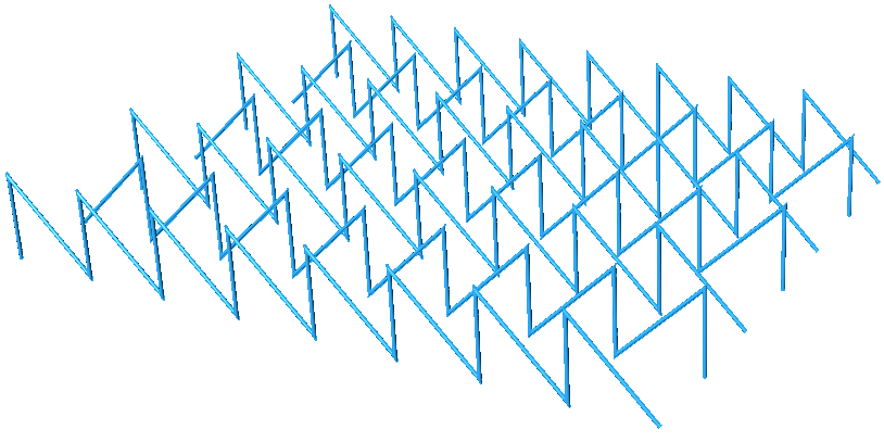
Solution... download GH file... Algorithm analysis: Since the zigzags alternate directions from one row to the next, it is best to split the grid into 2 parts, positive and negative. Find 3 sets of points in the positive tree and order Reverse the elements in the branches of the negative tree, then find the 3 sets of points and order Merge back the 2 trees to create geometry through points Grasshopper implementation: Use the Split Tree component to generate positive and negative trees for both bottom and top grids. Use {0,2,...} split mask. Use RelativeItems2 to create A and B trees, use {0}[+1] relative mask. Use Shift to create the C tree. Use Weave to combine data in the intended order, then remove consecutive duplicates using the DCon component. Merge ordered positive and negative trees to generate geometry using Polyline and Pipe components.

Tutorial 3.7.4: Truss
Create the structure shown in the image using a base grid as input.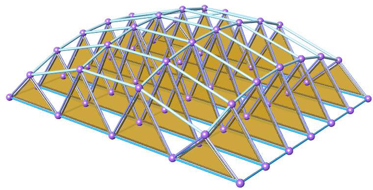
Solution... download GH file... Algorithm analysis: Understanding input: The 2 input grids with similar data structure (7 branches and with 9 elements). Bottom grid: Top grid: Understanding output: There are 4 parts to the output: 1. Bottom beams 2. Top beams 3. Middle beams 4. Middle plates Discussion: Constructing the bottom and top grids can be achieved with culling some points and flipping the points grid to get both directions. The middle beams weave the 2 culled grids of the bottom and top grids. We can also use the culled points to create the joints. Constructing the triangular connections is more involved since we need to create groups of 3 points that use a pair of consecutive points from the bottom grid and one point from the top. We can use relative trees to solve this. We can then offset the triangles to create the frame points, and offset again to create the plates points. Grasshopper implementation: Cull top and bottom tree, flip culled tree, then feed the 4 trees into a pipe component with the desired radius as a parameter Weave bottom and top grids to generate the grid of middle beams. Connect grid rows with a Polyline the use Pipe with the radius as a parameter To create the triangular connections, we will use a relative tree on the culled bottom grid, and combine with the culled top grid. Use Offset to generate smaller grid for the plates and their frame Offset the triangles to create desired sizes. Use Pipe and boundary to create frames and surfaces for the plates The full Grasshopper definition

Tutorial 3.7.5: Weaving
Create the structure shown in the image using a base grid as input.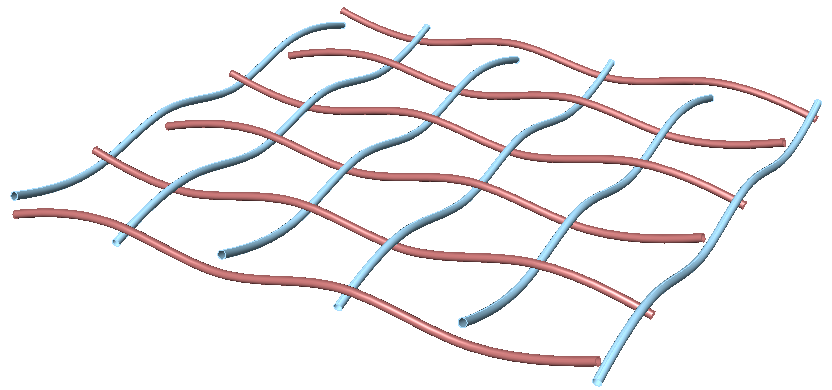
Solution... download GH file... Algorithm analysis: The input is a planar square grid with vertical branches. For vertical threads: Split the grid into two parts alternating elements in each branch. Move the first part up, and the second down, then recombine the parts into one set Draw a curve through the points in each branch. Flip the grid, then repeat to create horizontal curves Grasshopper implementation: Use Split Tree to separate alternating points and move up and down Combine points and use IntCrv to interpolate through points of each branch Flip the tree, and repeat Split, Combine and IntCrv to create curves in the other direction The full Grasshopper definition Expanded solution: Instead of using the Z-Axis to move points up and down, use the surface normal direction at each point Note: Make sure the data structure of normals and points match The Grasshopper definition:

End of guide

This is part 3-3 of the Essential Algorithms and Data Structures for Grasshopper.

Edit this page

Edit on GitHub

History

Admin